Introduction
The transformer architecture has become the foundation of modern deep learning, powering everything from language models to vision models. Since I’ll be referencing transformers frequently in future posts, I wanted to create my own comprehensive analysis of the architecture. In this post, I’ll walk through building a transformer-based translation model step by step, following the original paper by Vaswani et al. (2017)1. We’ll dive into the code, understanding each component as we implement it.
According to Vaswani et al. (2017), the transformer architecture was introduced as a translation model. It can be inferred from the paper that at the time of its introduction, RNN-based encoder-decoder architectures were commonly used for translation tasks. However, as you might know, RNN-based models compute sequentially, which limits parallelization.
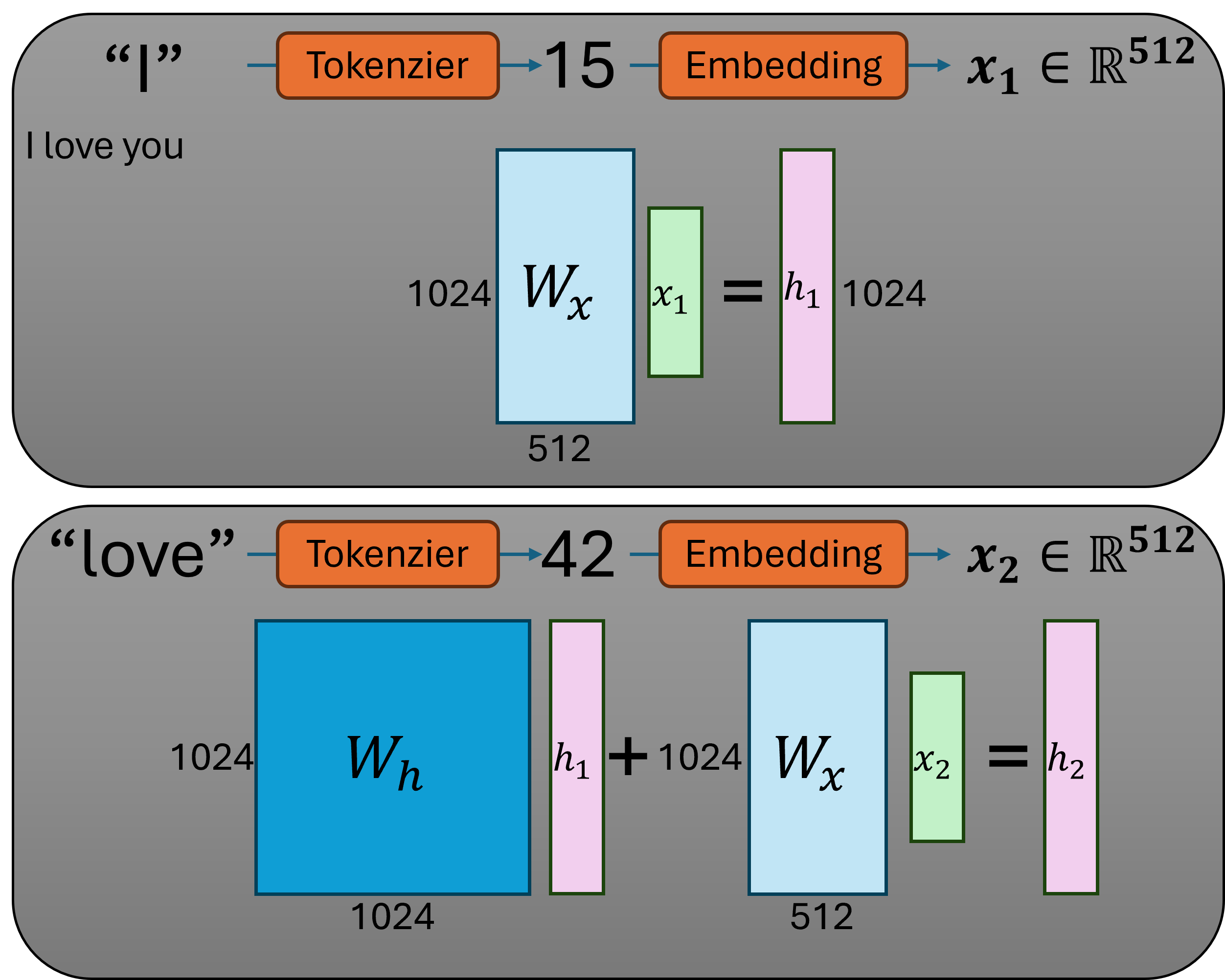
Figure 1 illustrates how an RNN processes a sequence. Take the input “I” from the phrase “I love you”: it is tokenized (e.g., to the id 15) and then passed through an embedding layer to obtain $x_1 \in \mathbb{R}^{512}$ (assuming embedding size 512). At this first time step there is no previous hidden state, so the model computes $h_1$ as $W_x x_1$, where $W_x \in \mathbb{R}^{1024 \times 512}$. The result is the hidden state $h_1 \in \mathbb{R}^{1024}$. For the next word “love”, the token (e.g., 42) is embedded to $x_2 \in \mathbb{R}^{512}$. The recurrence appears here: the new hidden state is $h_2 = W_h h_1 + W_x x_2$, where $W_h \in \mathbb{R}^{1024 \times 1024}$ is the recurrent weight. So at each step $t$, $h_t = W_h h_{t-1} + W_x x_t$ (with $h_0$ treated as zero or omitted at $t=1$). Bias terms are omitted in the figure and in the equations for simplicity.
Since RNNs were dominant at the time, attention mechanisms were mainly integrated into RNN-based architectures, which still suffered from sequential computation and limited scalability.
People also considered CNNs for language modeling, but CNNs can only see locally based on the kernel size, so it is difficult to learn dependencies between far-away words.
The Transformer architecture was introduced to overcome these constraints by eliminating recurrence and convolution, relying solely on attention mechanisms. This idea is reflected in the paper’s title, Attention Is All You Need.
The implementation in this post draws on the code at hkproj/pytorch-transformer2.
Big Picture
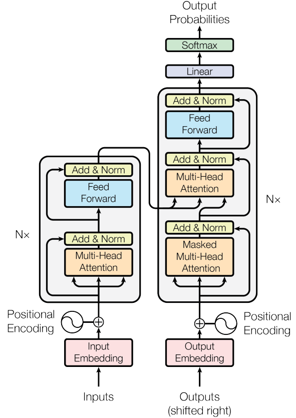
Left is the encoder and right is the decoder.
Consider the architecture as an English–Korean translator (because Korean is relatively easy for me). The encoder receives the English sentence “I love you.” The decoder does not take this sentence directly as input. Instead, it generates the Korean sentence autoregressively. Its inputs are the previously generated tokens, for example: ["
At each step, the decoder predicts the next token while attending to the encoder’s representations through cross-attention. No matter how long the input is, the encoder runs only once, and its output is fed into the decoder’s multi-head attention.
Encoder
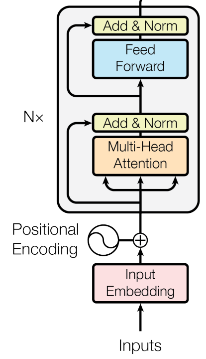
Input Embedding
Building Input Embedding is quite simple since Pytorch already made pre-built one.
class InputEmbedding(nn.Module):

    def __init__(self, d_model: int, vocab_size: int):
        super().__init__()
        self.d_model = d_model # dimension of the model (embedding size)
        self.vocab_size = vocab_size
        self.embedding = nn.Embedding(vocab_size, d_model)

    def forward(self, x):
        return self.embedding(x) * math.sqrt(self.d_model)
        # output: (batch_size, seq_len, d_model)
        # The output is then passed to the positional encoding layer.
The embedding layer must be trainable because the model needs to capture semantic relationships between words. Similar words should be positioned close to each other in the vector space, while dissimilar words should be placed farther apart.
For this reason, nn.Embedding is implemented as a parameter matrix (probably). Conceptually, it can be written in code as follows:
class Embedding(nn.Module):
    def __init__(self, vocab_size=10000, d_model=512):
        super().__init__()
        self.vocab_size = vocab_size
        self.d_model = d_model

        # (vocab_size, d_model) learnable parameter matrix
        self.W = nn.Parameter(torch.randn(vocab_size, d_model))

    def forward(self, x):
        # x: (batch_size, seq_len) containing token indices
        # return: (batch_size, seq_len, d_model)
        return self.W[x]
Anyway, for the practical use, Let’s stick to nn.Embedding, which must be implemented in more efficient way.
Also, In the paper, It says “In the embedding layers, we multiply those weights by $\sqrt{d_{model}}$.” But why? This is just my theory, but I think they probably initialized the embeddings with a normal distribution like $N(0,(1/\sqrt{d_{model}})^2)$. By multiplying the embeddings by $\sqrt{d_{model}}$, the resulting values would have a variance of 1, roughly matching the range of the positional encodings, which go from -1 to 1. This scaling helps balance the contributions of the embeddings and positional encodings in the model.
Since PyTorch’s nn.Embedding is already initialized as $N(0,1)$, I probably don’t need to multiply by $\sqrt{d_{model}}$ in this implementation. That scaling was mainly for the original initialization in the paper, which probably used a smaller variance. But let’s keep this setting for now and see how it works.
Positional Encoding
RNN has ordering feature, but this architecture is without RNN. So, Intuitively, It needs one feature for recognizing position of each token. It totally makes sense. Let’s see the way that the paper suggested. $$ PE_{pos,2i}=sin(\frac{pos}{10000^{\frac{2i}{d_{model}}}}), when\text{ } i:even$$ $$ PE_{pos,2i+1}=cos(\frac{pos}{10000^{\frac{2i}{d_{model}}}}), when\text{ } i:odd$$
So, it’s telling that first position’s positional vector would be like this : $$[sin(\frac{0}{10000^{\frac{2*0}{512}}}),cos(\frac{0}{10000^{\frac{2*0+1}{512}}}),…,sin(\frac{0}{10000^{\frac{2*255}{512}}}),cos(\frac{0}{10000^{\frac{2*255+1}{512}}})]$$ $$[0,1,…,0,1]$$ and second positional vector would be like: $$[sin(\frac{1}{10000^{\frac{2*0}{512}}}),cos(\frac{1}{10000^{\frac{2*0+1}{512}}}),…,sin(\frac{1}{10000^{\frac{2*255}{512}}}),cos(\frac{1}{10000^{\frac{2*255+1}{512}}})]$$
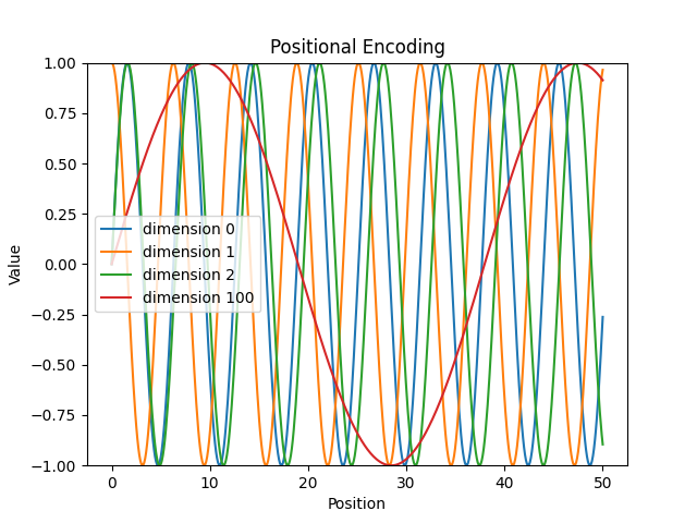
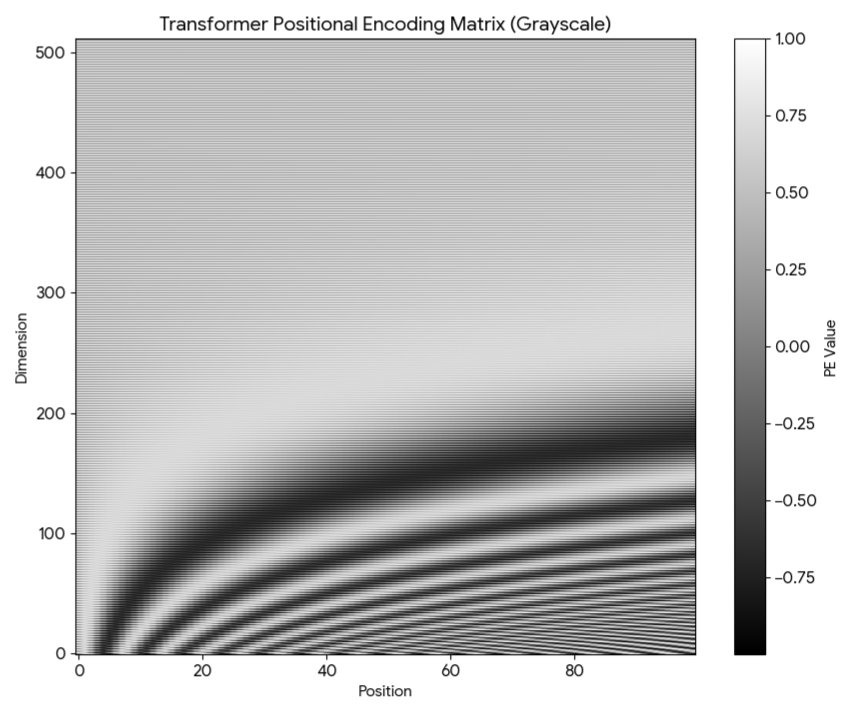
Based on the figures, it makes sense that every position can get a unique positional vector. The author presents a few benefits of it.
First, If we use a pair of sine and cosine (instead of using only one of them), we can represent the relationship between any two positions as a linear transformation (Rotation). This means that a function calculating the distance between position 2 and position 5 is linear and simple, making it easier for the model to find the function. Plus, the distance between position 2 and position 5 is the same as the distance between position 8 and position 11.
Second, This formulation enables the model to generalize to sequence lengths beyond those encountered during training. With learned positional embeddings (not this one), a model trained up to length 100 may struggle when encountering position 101, since it has never learned that index. In contrast, the sinusoidal formulation can generate a positional vector for any new position simply by plugging it into the formula.
Also, the values remain between -1 and 1, which is a great advantage when scaling.
About adding this positional encoding and input embedding, I thought positional encoding could harm the meaning of the words (Input Embeddings) by adding some noise. For example, I imagined “chimpanzee” at position 5 could be the same as “cat” at position 12. However, this post3 suggests an interesting possibility. As we saw in Figure 5, there is not that much difference after about dimension 200. So, the model might relatively avoid dimensions 0 to 200 and use dimesion atfer 200 when it forms input embeddings during training.
class PositionalEncoding(nn.Module):

    def __init__(self, d_model: int, max_seq_len: int, dropout: float):
        super().__init__()
        self.d_model = d_model
        self.max_seq_len = max_seq_len
        self.dropout = nn.Dropout(dropout)

        # (max_seq_len, d_model)
        pe = torch.zeros(max_seq_len, d_model)

        # (max_seq_len, 1)
        position = torch.arange(0, max_seq_len, dtype=torch.float32).unsqueeze(1)
        div_term = torch.exp(torch.arange(0, d_model, 2).float() * -(math.log(10000.0) / d_model))
        pe[:, 0::2] = torch.sin(position * div_term)
        pe[:, 1::2] = torch.cos(position * div_term)

        # (max_seq_len, d_model) -> (1, max_seq_len, d_model)
        pe = pe.unsqueeze(0)

        # Buffer: not a trainable parameter, but part of the model state
        # it will be saved and loaded with the model
        self.register_buffer('pe', pe)

    # x: (batch_size, seq_len, d_model)
    # x is the output of the input embedding layer.
    def forward(self, x):
        x = x + self.pe[:, :x.size(1), :]
        return self.dropout(x)
        # output: (batch_size, seq_len, d_model)
Multi-Head Attention
Okay, so far, our output from positional encoding has meaning of words and position information. Now, we need to add another feature for the model to understand the relationship between words. Attention will do the job.
.png)
Figure 7, which was originally from the paper, is a good visualization of attention, but let me explain it in a bit more detail.
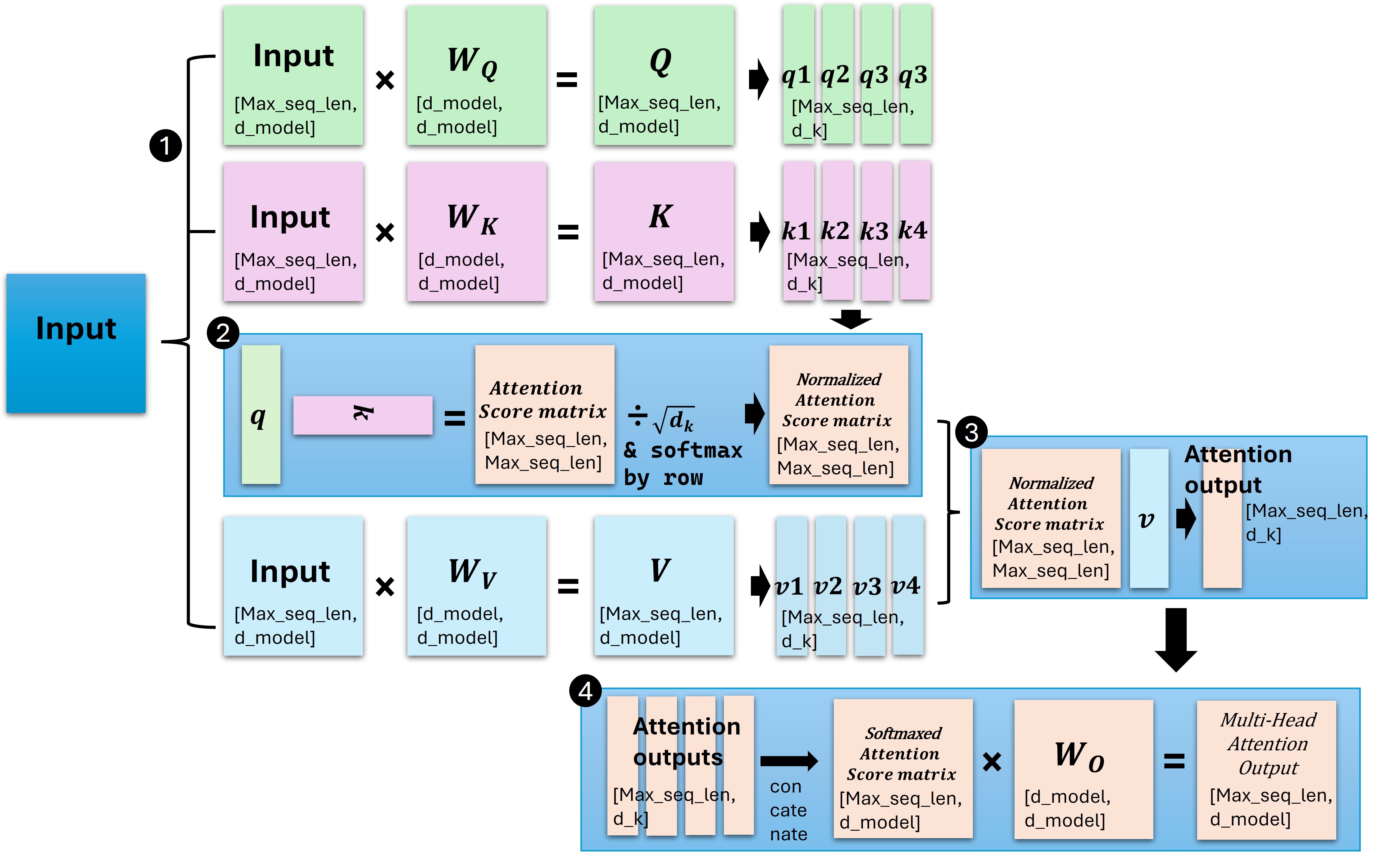
The objective of attention is to calculate the similarity between the query and the key, and then use the similarity to weight the value.
(1) First, we generate three matrices: $W_Q$, $W_K$, $W_V$, and multiply them with the input. The outputs are query $Q$, key $K$, and value $V$. The space of Q, K, V is [max_seq_len, d_model], which is same as the input embedding, positional encoding, and the sum of them. If we set the number of head to 4, for example, the space of Q, K, V would be [max_seq_len, 4, d_model/4]. d_model/4 is d_k and d_v(I didn’t use $d_v$ in the notation because $d_k$ and $d_v$ are the same in this case). Next, we transpose the head dimension and the sequence length dimension to obtain the shape [4, max_seq_len, d_model/4]. This allows each head to process the entire sequence independently and enables efficient batch computation across heads. So far, Q, K, and V are [4, max_seq_len, d_k].
At this point, although $W_Q$, $W_K$, and $W_V$ are different, Q, K, and V share the same architecture. There is no mechanism that differentiates their roles yet.
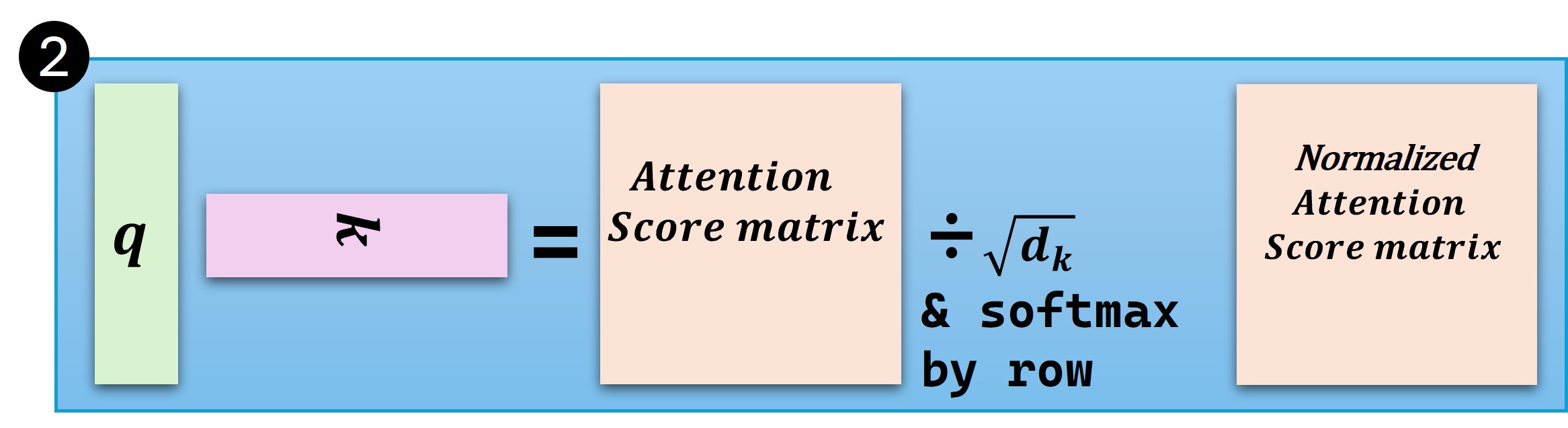
(2) Next, we dot product Q and K. The result is [4, max_seq_len, max_seq_len]. [max_seq_len, max_seq_len] is called attention score matrix. So, we have 4 attention score matrices. Then, we divide the attention score matrix by the square root of d_k before applying softmax. This is to prevent the dot product from becoming too large.
But why square root of d_k? The attention score matrix is computed by dot product of $Q$ and $K^T$, which is [4, max_seq_len, d_k] and [4, d_k, max_seq_len]. We can assume that the elements of Q and K are approximately independent and follow a normal distribution N(0,1) or at least constant variance.
So, the dot product of Q and K follows normal distribution N(0,d_k). So, the square root of d_k is to normalize the dot product, which leads to each sample of attention score matrix to be a random variable from normal distribution N(0,1).
Why do we want the dot product to follow a distribution close to N(0,1)? The reason is stability before applying softmax. If the variance of the dot product is large (i.e., proportional to d_k), the attention scores can contain very large positive and negative values. Since softmax involves exponentiation, large positive values will dominate, while large negative values will be pushed close to zero. As a result, the output distribution becomes extremely sharp, almost like a one-hot vector.
When softmax becomes too sharp, the gradients can become very small for most positions, making learning unstable or slow. By scaling the dot product by $\sqrt{d_k}$, we normalize its variance to 1. This keeps the softmax input values in a reasonable range and prevents the attention distribution from becoming overly peaked.
Finally, we apply a row-wise softmax to the attention score matrix. The resulting shape remains [4, max_seq_len, max_seq_len], but each row now represents a valid probability distribution. This step is crucial as it formally assigns distinct roles to Q and K: Q functions as the ‘query’ (the seeker), while K acts as the ‘key’ (the target).
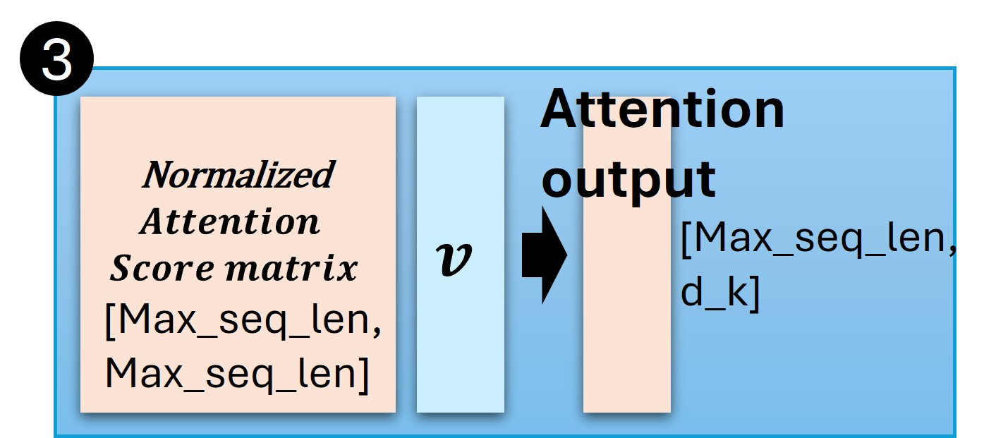
(3) This normalized attention score matrix [4, max_seq_len, max_seq_len] is then multiplied by V [4,max_seq_len, d_k] to get the final output. The shape remains [4, max_seq_len, d_k].
Why do we conceptually separate $V$ and multiply it at the end? The attention score matrix defines how strongly each query is related to every key. However, these scores only represent similarity—they do not contain the information itself. The matrix V provides the vectors that will be combined according to these similarity weights.
I think, this late-stage multiplication by $V$ serves a purpose similar to a residual connection within the attention mechanism itself. By keeping the “content” ($V$) separate from the “addressing logic” ($Q, K$), we ensure that the original information is not distorted or lost during the complex similarity computations. Instead of being completely overwritten, the values in $V$ are selectively combined based on the scores, which helps the model maintain a stable flow of information across layers. While it is possible for some information to “leak” into the scores, the designated role of $V$ is to provide a reliable, high-fidelity base of information that the model can “extract” and “mix” according to the guidance provided by $Q$ and $K$.
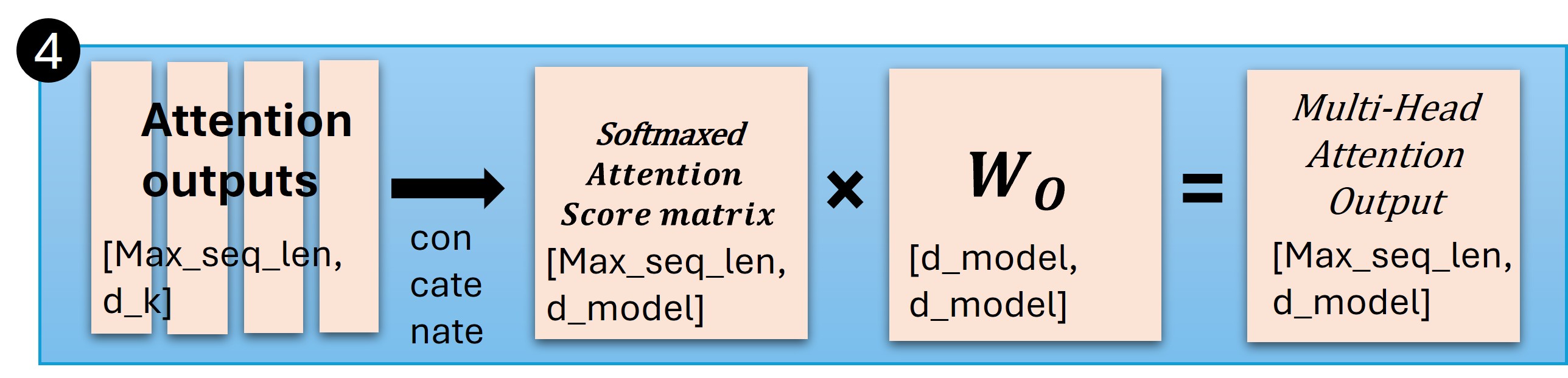
(4) Finally, we concatenate the outputs of the four heads and multiply by $W_O$ to get the final output. The shape remains [max_seq_len, d_model].
If we were to only concatenate the outputs, we would simply be laying out the information from the four independent heads side-by-side. At this stage, the insights captured by each head—hopefully different insights such as grammatical structures, semantic relationships, or distant dependencies—exist in isolation within their own subspaces.
By multiplying by $W_O$, we can combine the information from the four heads into a single matrix.
class MultiHeadAttentionBlock(nn.Module):

    def __init__(self, d_model: int, h: int, dropout: float):
        super().__init__()
        # dimension of the model
        self.d_model = d_model
        # number of heads
        self.h = h
        assert d_model % h == 0, "d_model must be divisible by h"

        # d_model = h * d_k
        self.d_k = d_model // h

        # weights for the query, key, and value matrices
        self.w_q = nn.Linear(d_model, d_model) # Wq
        self.w_k = nn.Linear(d_model, d_model) # Wk
        self.w_v = nn.Linear(d_model, d_model) # Wv

        # weights for the output matrix
        self.w_o = nn.Linear(d_model, d_model) # Wo
        self.dropout = nn.Dropout(dropout)

    # query: (batch_size, h, max_seq_len, d_k)
    # key: (batch_size, h, max_seq_len, d_k)
    # value: (batch_size, h, max_seq_len, d_k)
    # mask: (batch_size, h, max_seq_len, max_seq_len)
    # dropout: dropout rate
    @staticmethod # static method: not bound to an instance, but to the class
    def attention(query, key, value, mask=None, dropout=None):
        d_k = query.shape[-1]

        # (batch_size, h, max_seq_len, d_k) @ (batch_size, h, d_k, max_seq_len) -> (batch_size, h, max_seq_len, max_seq_len)
        attention_scores = (query @ key.transpose(-2, -1)) / math.sqrt(d_k)
        if mask is not None:
            attention_scores = attention_scores.masked_fill(mask == 0, -1e9)
        # dim=-1: softmax over the last dimension
        attention_scores = attention_scores.softmax(dim=-1) # (batch_size, h, max_seq_len, max_seq_len)
        if dropout is not None:
            attention_scores = dropout(attention_scores)

        # (batch_size, h, max_seq_len, max_seq_len) @ (batch_size, h, max_seq_len, d_k) -> (batch_size, h, max_seq_len, d_k)
        return (attention_scores @ value), attention_scores # the latter is only for visualization

    def forward(self, q, k, v, mask=None):
        query = self.w_q(q) # (batch_size, max_seq_len, d_model) -> (batch_size, max_seq_len, d_model)
        key = self.w_k(k) # (batch_size, max_seq_len, d_model) -> (batch_size, max_seq_len, d_model)
        value = self.w_v(v) # (batch_size, max_seq_len, d_model) -> (batch_size, max_seq_len, d_model)

        # split the query, key, and value into h heads
        # (batch_size, max_seq_len, d_model) -> (batch_size, max_seq_len, h, d_k) -> (batch_size, h, max_seq_len, d_k)
        query = query.view(query.shape[0], query.shape[1], self.h, self.d_k).transpose(1, 2)
        key = key.view(key.shape[0], key.shape[1], self.h, self.d_k).transpose(1, 2)
        value = value.view(value.shape[0], value.shape[1], self.h, self.d_k).transpose(1, 2)


        x, self.attention_scores = MultiHeadAttentionBlock.attention(query, key, value, mask, self.dropout)
        # output x: (batch_size, h, max_seq_len, d_k)

        # (batch_size, h, max_seq_len, d_k) -> (batch_size, max_seq_len, h, d_k) --> (batch_size, max_seq_len, d_model)
        batch_size, _, seq_len, _ = x.size()
        x = x.transpose(1, 2).contiguous().reshape(batch_size, seq_len, self.d_model)

        # (batch_size, max_seq_len, d_model) -> (batch_size, max_seq_len, d_model)
        return self.w_o(x)
Let’s see the implementation of the multi-head attention block. In the forward method, we take the query, key, and value as input.
But, isn’t it weird that we take the query, key, and value seperatly? In self-attention, the query, key, and value are all derived from the same input.So why not simply pass a single tensor instead? The reason is flexibility. While self-attention uses the same input to generate Q, K, and V, other forms of attention—such as cross-attention in the decoder—use different sources. In cross-attention, the query comes from the decoder, whereas the key and value come from the encoder output.
By accepting query, key, and value separately, this implementation remains general and can be reused for both self-attention and cross-attention.
query = self.w_q(q) # (batch_size, max_seq_len, d_model) -> (batch_size, max_seq_len, d_model)
key = self.w_k(k) # (batch_size, max_seq_len, d_model) -> (batch_size, max_seq_len, d_model)
value = self.w_v(v) # (batch_size, max_seq_len, d_model) -> (batch_size, max_seq_len, d_model)
After above operations, Q, K, and V matrices are generated.
# (batch_size, max_seq_len, d_model) -> (batch_size, max_seq_len, h, d_k) -> (batch_size, h, max_seq_len, d_k)
query = query.view(query.shape[0], query.shape[1], self.h, self.d_k).transpose(1, 2)
key = key.view(key.shape[0], key.shape[1], self.h, self.d_k).transpose(1, 2)
value = value.view(value.shape[0], value.shape[1], self.h, self.d_k).transpose(1, 2)
query.shape[0] is batch_size, query.shape[1] is max_seq_len, self.h is number of heads, self.d_k is dimension of the key (and value). Of course, self.h * self.d_k is d_model. If our d_model is 512 and we set the number of heads to 8, self.d_k is 64. Because first two dimensions are batch_size and max_seq_len, which is same as the before, the view operation is just to split the d_model dimension into h heads. [batch_size, max_seq_len, h, d_k].
Next, we transpose the head dimension and the sequence length dimension to obtain the shape [h, batch_size, max_seq_len, d_k]. This allows each head to process the entire sequence independently and enables efficient batch computation across heads.
    # query: (batch_size, h, max_seq_len, d_k)
    # key: (batch_size, h, max_seq_len, d_k)
    # value: (batch_size, h, max_seq_len, d_k)
    # mask: (batch_size, h, max_seq_len, max_seq_len)
    # dropout: dropout rate
    @staticmethod # static method: not bound to an instance, but to the class
    def attention(query, key, value, mask=None, dropout=None):
        d_k = query.shape[-1]

        # (batch_size, h, max_seq_len, d_k) @ (batch_size, h, d_k, max_seq_len) -> (batch_size, h, max_seq_len, max_seq_len)
        attention_scores = (query @ key.transpose(-2, -1)) / math.sqrt(d_k)
        if mask is not None:
            attention_scores = attention_scores.masked_fill(mask == 0, -1e9)
        # dim=-1: softmax over the last dimension
        attention_scores = attention_scores.softmax(dim=-1) # (batch_size, h, max_seq_len, max_seq_len)
        if dropout is not None:
            attention_scores = dropout(attention_scores)

        # (batch_size, h, max_seq_len, max_seq_len) @ (batch_size, h, max_seq_len, d_k) -> (batch_size, h, max_seq_len, d_k)
        return (attention_scores @ value), attention_scores # the latter is only for visualization
x, self.attention_scores = MultiHeadAttentionBlock.attention(query, key, value, mask, self.dropout)
# output x: (batch_size, h, max_seq_len, d_k)
# self.attention_scores: (batch_size, h, max_seq_len, max_seq_len)
By calling the attention function, we get the output x and the attention scores. x is the outout of (3) in Figure 10. [batch_size, h, max_seq_len, d_k].
Mask for Encoder is called padding mask. If the token is padding, the attention score is set to -1e9. If max_seq_len is 5, and ‘I’, ’love’, ‘you’ are the tokens, then the mask is : $$ \begin{bmatrix} 1 & 1 & 1 & 0 & 0 \\ 1 & 1 & 1 & 0 & 0 \\ 1 & 1 & 1 & 0 & 0 \\ 1 & 1 & 1 & 0 & 0 \\ 1 & 1 & 1 & 0 & 0 \end{bmatrix} $$ However, at first glance, I thought that the mask should be like this: $$ \begin{bmatrix} 1 & 1 & 1 & 0 & 0 \\ 1 & 1 & 1 & 0 & 0 \\ 1 & 1 & 1 & 0 & 0 \\ 0 & 0 & 0 & 0 & 0 \\ 0 & 0 & 0 & 0 & 0 \end{bmatrix} $$ Because [4,1] and other elements are also related to padding. But it was not a case. The reason we use the first mask instead of the second lies in computational efficiency and the independent nature of the Transformer layers.
First, using a uniform mask across all rows allows for Broadcasting. Instead of creating a complex, row-specific mask, the hardware can simply broadcast a single $[1 \times 5]$ vector across the entire matrix. This significantly speeds up the operation on modern GPUs.
Second, you might worry that these “garbage” padding rows (rows 4 and 5) will eventually pollute the actual information in rows 1 to 3. However, this doesn’t happen because the subsequent layers—$W_O$ and the Feed Forward Network (FFN)—process each row independently.
Since these layers do not mix information across different rows, the noise in the padding rows stays trapped within those rows. As long as we have masked the Keys (columns) to prevent real tokens from looking at padding, the real tokens remain pure. Therefore, we can simply ignore these padding rows at the very end of the model or during loss calculation, making a dedicated row-wise mask unnecessary during the encoding process.
# (batch_size, h, max_seq_len, d_k) -> (batch_size, max_seq_len, h, d_k) --> (batch_size, max_seq_len, d_model)
x = x.transpose(1,2).contiguous().view(x.shape[0], x.shape[1], self.h * self.d_k)
By transposing the head dimension and the sequence length dimension, we get the shape [batch_size, max_seq_len, h, d_k]. Then, we concatenate the heads and get the shape [batch_size, max_seq_len, d_model] again.
return self.w_o(x)
Finally, we multiply by $W_O$ to get the final output, which is the output of (4) in Figure 11, which is Multi-Head Attention Output. So, the shape is [batch_size, max_seq_len, d_model].
Residual Connection and Layer Normalization
Now, it’s time to make the Add & Norm part, which is a residual connection and layer normalization. First, Let’s see the layer normalization4.
$$LN(x)=\alpha\frac{x-\mu}{\sqrt{\sigma^2+\epsilon}}+\beta$$
class LayerNormalization(nn.Module):

    def __init__(self, d_model: int, eps: float = 1e-6):
        super().__init__()
        self.eps = eps

        # learnable parameters
        self.alpha = nn.Parameter(torch.ones(d_model)) # scale
        self.bias = nn.Parameter(torch.zeros(d_model)) # shift

    # x: (batch_size, max_seq_len, d_model)
    def forward(self, x):
        # (batch_size, max_seq_len, d_model) -> (batch_size, max_seq_len, 1)
        mean = x.mean(dim=-1, keepdim=True)
        # (batch_size, max_seq_len, d_model) -> (batch_size, max_seq_len, 1)
        variance = x.var(dim=-1, keepdim=True)
        # (batch_size, max_seq_len, 1) -> (batch_size, max_seq_len, d_model)
        return self.alpha * (x - mean) / torch.sqrt(variance + self.eps) + self.bias
Whatever the input is, its shape is typically [batch_size, max_seq_len, d_model]. From the code, we can see that the mean and variance are computed along the last dimension (dim=-1). In other words, normalization is performed token-wise. Each token vector is normalized independently from other tokens in the same sequence. This means that :
- Each token’s representation is centered and scaled on its own.
- There is no statistical interaction across tokens during normalization.
- The normalization process does not introduce cross-token dependency.
If we computed the mean and variance along the sequence dimension instead (i.e., column-wise normalization), the normalization statistics would depend on other tokens in the sequence. That would make the representation of one token partially dependent on the values of other tokens through the normalization step itself. Such cross-token coupling is undesirable because:
- It entangles token representations.
- It may interfere with autoregressive decoding.
- It makes the representation less locally stable.
Transformer models are designed so that interactions between tokens occur explicitly through attention, not implicitly through normalization.
Also, The decisive reason LayerNorm is needed lies in the residual structure: $$x+Sublayer(x)$$
This residual connection continuously adds new signals to the original representation. If this process is repeated across many layers, the variance of activations can grow uncontrollably. Whitout normalization:
- The magnitude of activations may explode.
- Gradient flow can become unstable.
- Training deep stacks becomes difficult.
Layer normalization stabilizes this process by controlling the scale of the combined signal. $$LayerNorm(x+Sublayer(x))$$
Thus, LayerNorm acts as a variance regulator that keeps the representation well-conditioned throughout deep residual stacking.
In addition, LayerNorm includes two learnable parameters, $\alpha$ (scale) and $\beta$ (shift). After normalization forces the representation to have zero mean and unit variance, these parameters allow the model to re-scale and re-shift the normalized output.
Without $\alpha$ and $\beta$, normalization would strictly constrain every token representation to the same standardized distribution. However, such rigid normalization could limit the expressive power of the network. By introducing learnable scale and shift parameters, the model can recover any necessary distribution if needed, while still benefiting from stabilized training.
In other words, LayerNorm first standardizes the representation for numerical stability, and then $\alpha$ and $\beta$ give the model the flexibility to learn the most useful scaling for downstream computation. After the affine transformation, the output has mean approximately $\beta$ and variance approximately $\alpha^2$ (per token), but it is not necessarily Gaussian.
Now, Let’s see the complete Add & Norm part.
class ResidualConnection(nn.Module):

    def __init__(self, d_model: int, dropout: float):
        super().__init__()
        self.dropout = nn.Dropout(dropout)
        self.norm = LayerNormalization(d_model)

    def forward(self, x, sublayer):
        return self.norm(x + self.dropout(sublayer(x)))
Here, sublayer is a function and can represent any layer, such as a multi-head attention block or a feed-forward network.
Since layer normalization is applied after adding the residual connection, this structure is called Post-LN. Although this follows the original formulation in the paper, more recent implementations often use the Pre-LN variant.
$$x+Sublayer(LayerNorm(x))$$
class ResidualConnection(nn.Module):

    def __init__(self, d_model: int, dropout: float):
        super().__init__()
        self.dropout = nn.Dropout(dropout)
        self.norm = LayerNormalization(d_model)

    def forward(self, x, sublayer):
        return x + self.dropout(sublayer(self.norm(x)))
In the Pre-LN structure, layer normalization is applied before the sublayer. Apprently, this design leads to more stable gradient flow and tends to work better in deeper models.
Feed-Forward
The last part to implement is the feed-forward network.
class FeedForwardBlock(nn.Module):

    def __init__(self, d_model: int, d_ff: int, dropout: float):
        super().__init__()
        self.linear_1 = nn.Linear(d_model, d_ff) # W1 and b1
        self.linear_2 = nn.Linear(d_ff, d_model) # W2 and b2
        self.dropout = nn.Dropout(dropout)
        self.d_model = d_model

    def forward(self, x):
        # (batch_size, max_seq_len, d_model) -> (batch_size, max_seq_len, d_ff) -> (batch_size, max_seq_len, d_model)
        return self.linear_2(self.dropout(torch.relu(self.linear_1(x))))
Just simply two linear layers and a dropout. But why we use Feed-Forward block? isn’t attention blocks enough?
The key difference is that attention mixes information across tokens, while the feed-forward network transforms each token representation independently. Attention allows each position to gather relevant information from the sequence, but it is mostly a weighted linear combination of value vectors. Without an additional non-linear transformation, the model’s expressive power would be limited.
The feed-forward block provides this non-linearity and increases the representational capacity of the model (There were no non-linearities at all before feed-forward!). After attention aggregates contextual information, the feed-forward network processes and refines that information at each position. In this way, attention handles interaction between tokens, and the feed-forward block performs deeper feature transformation.
Encoder Block
Now, let’s see the complete encoder block. It’s just a combination of all the parts we’ve seen so far.
class EncoderBlock(nn.Module):

    def __init__(self, d_model: int, self_attention_block: MultiHeadAttentionBlock, feed_forward_block: FeedForwardBlock, dropout: float):
        super().__init__()
        self.self_attention_block = self_attention_block
        self.feed_forward_block = feed_forward_block
        # two residual connections: one for the self-attention block and one for the feed-forward block
        self.residual_connections = nn.ModuleList([ResidualConnection(d_model, dropout) for _ in range(2)])

    # source_mask is needed because the encoder needs to know what positions are valid and which are not.
    # 'not valid' means that the position is padding
    def forward(self, x, source_mask=None):
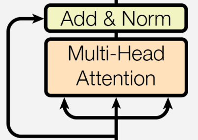
        x = self.residual_connections[0](x, lambda x: self.self_attention_block(x, x, x, source_mask))
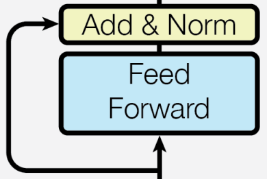
        x = self.residual_connections[1](x, self.feed_forward_block)
        return x
The code is quite straightforward. The first line of the forward method is exactly here :
And the second line is also exactly here :
Finally, In the paper, we need to repeat the encoder block N times.
class Encoder(nn.Module):

    def __init__(self, d_model: int, layers: nn.ModuleList):
        super().__init__()
        self.layers = layers
        self.norm = LayerNormalization(d_model)

    def forward(self, x, mask):
        for layer in self.layers:
            x = layer(x, mask)
        return self.norm(x)
layers is a list of encoder blocks. As you can see, we apply layer normalization after the last encoder block.
Decoder
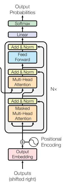
We built most of classes for decoder block during building encoder, so we can immediately go to DecoderBlock.
Decoder Block
class DecoderBlock(nn.Module):

    def __init__(self, d_model: int, self_attention_block: MultiHeadAttentionBlock, cross_attention_block: MultiHeadAttentionBlock, feed_forward_block: FeedForwardBlock, dropout: float):
        super().__init__()
        self.self_attention_block = self_attention_block
        self.cross_attention_block = cross_attention_block
        self.feed_forward_block = feed_forward_block
        self.residual_connections = nn.ModuleList([ResidualConnection(d_model, dropout) for _ in range(3)])


    def forward(self, x, encoder_output, source_mask, target_mask):
        x = self.residual_connections[0](x, lambda x: self.self_attention_block(x, x, x, target_mask))
        x = self.residual_connections[1](x, lambda x: self.cross_attention_block(x, encoder_output, encoder_output, source_mask))
        x = self.residual_connections[2](x, self.feed_forward_block)
        return x
Let’s see the first line of the forward method :
x = self.residual_connections[0](x, lambda x: self.self_attention_block(x, x, x, target_mask))
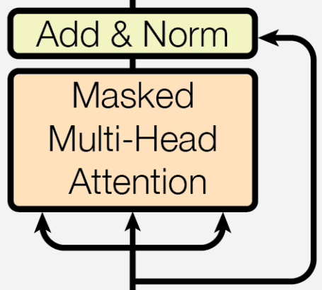
In this step, we use a target mask instead of a source mask. In the context of this translator, the source mask is applied to the source language (English), while the target mask is for the target language (Korean). The source mask masks padding tokens in the source sequence. The target mask, however, not only masks padding tokens but also blocks access to future tokens to preserve the autoregressive property of the decoder.
If the maximum sequence length is 5 and the input tokens are “I”, “love”, and “you”, the source sequence becomes: [“I”, “love”, “you”, “<PAD>”, “<PAD>”]
Suppose the corresponding output tokens are “나는”, “너를”, and “사랑해”. During training, the decoder input would be: ["<SOS>", “나는”, “너를”, “사랑해”, “<PAD>”]
To prevent the model from attending to future tokens, we first apply a causal (look-ahead) mask of the following form: $$ \begin{bmatrix} 1 & 0 & 0 & 0 & 0 \\ 1 & 1 & 0 & 0 & 0 \\ 1 & 1 & 1 & 0 & 0 \\ 1 & 1 & 1 & 1 & 0 \\ 1 & 1 & 1 & 1 & 1 \end{bmatrix} $$
However, this is not sufficient, because the last position corresponds to a padding token. Therefore, we additionally mask the padding position, resulting in the final target mask: $$ \begin{bmatrix} 1 & 0 & 0 & 0 & 0 \\ 1 & 1 & 0 & 0 & 0 \\ 1 & 1 & 1 & 0 & 0 \\ 1 & 1 & 1 & 1 & 0 \\ 1 & 1 & 1 & 1 & 0 \end{bmatrix} $$
In this way, the decoder attends only to previously generated tokens and ignores padding positions.
And here, second line of the forward method :
x = self.residual_connections[1](x, lambda x: self.cross_attention_block(x, encoder_output, encoder_output, source_mask))
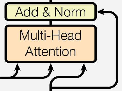
In this cross-attention step, the query comes from the decoder’s current hidden state $x$, while both the key and value come from the encoder output. This design reflects the role of cross-attention: the decoder queries the encoded source representation to retrieve relevant information for generating the next target token. Since the goal is to produce a target-side representation for each decoder position, the output length must match the target sequence length. Therefore, the decoder provides the queries, and the encoder provides the keys and values.
Also, the mask must match the key sequence. Since the keys and values come from the encoder output, we apply the source mask to prevent the decoder from attending to padded positions in the source sequence. The target mask is not used here because cross-attention does not involve future target tokens.
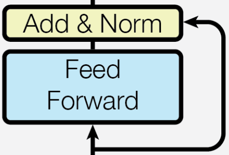
Last, third line of the forward method is feed-forward.
x = self.residual_connections[2](x, self.feed_forward_block)
Now, we repeat the decoder block N times.
class Decoder(nn.Module):

    def __init__(self, d_model: int, layers: nn.ModuleList):
        super().__init__()
        self.layers = layers
        self.norm = LayerNormalization(d_model)

    def forward(self, x, encoder_output, source_mask, target_mask):
        for layer in self.layers:
            x = layer(x, encoder_output, source_mask, target_mask)
        return self.norm(x)
Projection Layer
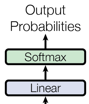
Projection Layer is a simple linear layer that projects the decoder output to the vocabulary size.
class ProjectionLayer(nn.Module):

    def __init__(self, d_model: int, vocab_size: int):
        super().__init__()
        self.proj = nn.Linear(d_model, vocab_size)

    def forward(self, x):
        # (batch_size, max_seq_len, d_model) -> (batch_size, max_seq_len, vocab_size)
        return torch.log_softmax(self.proj(x), dim=-1)
Complete Transformer
class Transformer(nn.Module):

    def __init__(self, encoder: Encoder, decoder: Decoder, src_embed: InputEmbedding, tgt_embed: InputEmbedding, src_pos: PositionalEncoding, tgt_pos: PositionalEncoding, projection_layer: ProjectionLayer):
        super().__init__()
        self.encoder = encoder
        self.decoder = decoder
        self.src_embed = src_embed
        self.tgt_embed = tgt_embed
        self.src_pos = src_pos
        self.tgt_pos = tgt_pos
        self.projection_layer = projection_layer

    def encode(self, src_sequence, src_mask):
        x = self.src_embed(src_sequence)
        x = self.src_pos(x)
        return self.encoder(x, src_mask)

    def decode(self, tgt_sequence, encoder_output, src_mask, tgt_mask):
        x = self.tgt_embed(tgt_sequence)
        x = self.tgt_pos(x)
        return self.decoder(x, encoder_output, src_mask, tgt_mask)

    def project(self, x):
        return self.projection_layer(x)
We could just use forward method, but in this way, we can get more flexibility.
def build_transformer(src_vocab_size: int, tgt_vocab_size: int, src_seq_len: int, tgt_seq_len: int, d_model: int = 512, N: int = 6, h: int = 8, dropout: float = 0.1, d_ff: int = 2048):
    src_embed = InputEmbedding(d_model, src_vocab_size)
    tgt_embed = InputEmbedding(d_model, tgt_vocab_size)

    src_pos = PositionalEncoding(d_model, src_seq_len, dropout)
    tgt_pos = PositionalEncoding(d_model, tgt_seq_len, dropout)

    # Create the encoder blocks
    encoder_blocks = []
    for _ in range(N):
        encoder_self_attention_block = MultiHeadAttentionBlock(d_model, h, dropout)
        encoder_feed_forward_block = FeedForwardBlock(d_model, d_ff, dropout)
        encoder_blocks.append(EncoderBlock(d_model, encoder_self_attention_block, encoder_feed_forward_block, dropout))

    # Create the decoder blocks
    decoder_blocks = []
    for _ in range(N):
        decoder_self_attention_block = MultiHeadAttentionBlock(d_model, h, dropout)
        decoder_cross_attention_block = MultiHeadAttentionBlock(d_model, h, dropout)
        decoder_feed_forward_block = FeedForwardBlock(d_model, d_ff, dropout)
        decoder_blocks.append(DecoderBlock(d_model, decoder_self_attention_block, decoder_cross_attention_block, decoder_feed_forward_block, dropout))

    # Create the encoder and decoder
    encoder = Encoder(d_model, nn.ModuleList(encoder_blocks))
    decoder = Decoder(d_model, nn.ModuleList(decoder_blocks))

    # Create the projection layer
    projection_layer = ProjectionLayer(d_model, tgt_vocab_size)

    # Create the transformer
    transformer = Transformer(encoder, decoder, src_embed, tgt_embed, src_pos, tgt_pos, projection_layer)

    # Initialize the transformer
    for p in transformer.parameters():
        if p.dim() > 1:
            nn.init.xavier_uniform_(p)

    return transformer
To use the transformer, first we need to initialize the parts of the transformer. That’s why we have build_transformer function.
Here, why we use xavier initialization? Xavier initialization is a popular method for initializing the weights of a neural network. It is named after Xavier Glorot and Yoshua Bengio, who introduced it in their 2010 paper “Understanding the difficulty of training deep feedforward neural networks.”5
First, Let’s see forward propagation. Let’s say one layer is y. $$ y = Wx $$
- x $\in \mathbb{R}^{n}$
- W $\in \mathbb{R}^{m \times n}$
So, $y \in \mathbb{R}^{m}$.
Here,
nis called fan_in andmis called fan_out.single neuron in y : $y_i = \sum_{j=1}^{n} W_{i,j} x_j$.
Let’s say that Var($x_i$) = $\sigma^2_x$ and Var($W_{i,j}$) = $\sigma^2_w$.
Assume that :
- all $x_i$ are independent,
- all $W_{i,j}$ are independent,
- x_j and W_{i,j} are independent,
- and their means are 0.
Then the variance of $y_i$ is : First, recall that for random variables $Z_j$: $$ Var(\sum_{j=1}^{n} Z_j) = \sum_{j=1}^{n} Var(Z_j) + 2 \sum_{j < k} Cov(Z_j, Z_k) $$ If the terms are independent, all covariance terms vanish: $$Cov(Z_j, Z_k) = 0$$ Therefore, $$ Var(y_i) = Var(\sum_{j=1}^{n} W_{i,j} x_j) = \sum_{j=1}^{n} Var(W_{i,j} x_j) $$
Now, consider a single term $W_{i,j} x_j$. For two independent random variables A and B with zero mean: $$ Var(AB)=E(A^2)E(B^2)-E(A)^2E(B)^2$$ Since E(A)=E(B)=0, this simplifies to: $$ Var(AB)=E(A^2)E(B^2)=Var(A)Var(B)$$ Applying this to $W_{i,j} and x_j$, we get: $$ Var(W_{i,j} x_j) = Var(W_{i,j}) Var(x_j) = \sigma^2_w \sigma^2_x $$ Therefore, $$ Var(y_i) = \sum_{j=1}^{n} \sigma^2_w \sigma^2_x = n \sigma^2_w \sigma^2_x $$
If the number of layers is L, then the variance of the last layer is : $$ Var(y_L) \approx (n \sigma^2_w)^L $$
In this situation, if n \sigma^2_w is larger than 1, the variance will explode. If it is smaller than 1, the variance will vanish. So, we want to set $n \sigma^2_w$ to 1. $$ n \sigma^2_w = 1 $$ $$ \sigma^2_w = \frac{1}{n} = \frac{1}{fan_{in}} $$
Now, What about backward propagation? We want to compute the gradient with respect to the input: $$\frac{\partial L}{\partial x} \in \mathbb{R}^{n}$$ From forward propagation: $$y = Wx$$ By the chain rule, $$\frac{\partial L}{\partial x} =(\frac{\partial y}{\partial x})^{T} \frac{\partial L}{\partial y} = W^{T} \frac{\partial L}{\partial y}$$ Since $\frac{\partial y}{\partial x} = W$, we have: $$\frac{\partial L}{\partial x} = W^{T} \frac{\partial L}{\partial y}$$ Let $\delta y = \frac{\partial L}{\partial y}$, then: $$\delta x = W^{T} \delta y$$ For a single component: $$\delta x_i = \sum_{j=1}^{m} W_{i,j} \delta y_j$$ Assume:
- $Var(\delta y_j) = \sigma^2_{\delta}$
- $Var(W_{i,j}) = \sigma^2_w$
Then, $$ Var(\delta x_i) = \sum_{j=1}^{m} Var(W_{i,j} \delta y_j) = m \sigma^2_w \sigma^2_{\delta} $$
If the number of layers is L, then the variance of the last layer is : $$ Var(\delta x_L) \approx (m \sigma^2_w)^L \sigma^2_{\delta} $$ In this situation, if $m \sigma^2_w$ is larger than 1, the variance will explode. If it is smaller than 1, the variance will vanish. So, we want to set $m \sigma^2_w$ to 1. $$ m \sigma^2_w = 1 $$ $$ \sigma^2_w = \frac{1}{m} = \frac{1}{fan_{out}} $$
Forward stability requires $\sigma^2_w = \frac{1}{fan_{in}}$ and backward stability requires $\sigma^2_w = \frac{1}{fan_{out}}$. To balance both, Xavier initialization uses: $$ \sigma^2_w = \frac{2}{fan_{in} + fan_{out}} $$
So, if we put these sample from normal distribution, then it’s like this : $$ W_{i,j} \sim N(0, \frac{2}{fan_{in} + fan_{out}}) $$
However, if we want to put samples from uniform distribution, we need little more thinking. Uniform is like this : $$ W_{i,j} \sim U(-a,a) $$ The variance is : $$ Var(U) = \frac{a^2}{3} $$ and we want this to be equal to $\frac{2}{fan_{in} + fan_{out}}$.
$$ \frac{a^2}{3} = \frac{2}{fan_{in} + fan_{out}} $$ $$ a = \sqrt{\frac{6}{fan_{in} + fan_{out}}} $$
Xavier initialization fundamentally aims to control the variance of the weights; the choice between a normal and a uniform distribution is secondary. A normal distribution concentrates values around zero but still allows rare large values due to its tails, whereas a uniform distribution samples weights evenly within a fixed range and strictly prevents extreme values. In other words, the uniform version eliminates the possibility of unusually large initial weights. In practice, both approaches work well, but uniform initialization is often slightly preferred for its bounded range and empirical stability, which is why xavier_uniform_ is commonly used in PyTorch.
Using the transformer
Okay, now we will train the transformer and use it to translate English to Korean. For this, I will make dataset.py , config.py, and train.py files.
Dataset
Like every other torch implementation, we need to prepare the dataset module.
class BilingualDataset(Dataset):
    def __init__(self, ds, tokenizer_src, tokenizer_tgt, src_lang, tgt_lang, max_seq_len):
        super().__init__()

        # raw dataset
        self.ds = ds
        self.max_seq_len = max_seq_len # maximum sequence length
        self.tokenizer_src = tokenizer_src # tokenizer for the source language
        self.tokenizer_tgt = tokenizer_tgt # tokenizer for the target language
        self.src_lang = src_lang # source language, e.g. "english"
        self.tgt_lang = tgt_lang # target language, e.g. "korean"


        # special tokens
        # we pre-define the special tokens, so that we can use them in the getitem method.
        # If we keep calling torch.tensor([tokenizer.token_to_id("[SOS]")]) in the getitem method, it will be slow.
        self.sos_token = torch.tensor([tokenizer_src.token_to_id("[SOS]")], dtype=torch.int64) # start of sequence token.
        self.eos_token = torch.tensor([tokenizer_src.token_to_id("[EOS]")], dtype=torch.int64) # end of sequence token
        self.pad_token = torch.tensor([tokenizer_src.token_to_id("[PAD]")], dtype=torch.int64) # padding token
        # shape is (1,), dtype is int64

    def __len__(self):
        return len(self.ds) # return the length of the dataset

    def __getitem__(self, idx):
        src_target_pair = self.ds[idx] # get the source and target text from the dataset

        src_text = src_target_pair[self.src_lang] # get the source text from the dataset
        # e.g. "I love you"

        tgt_text = src_target_pair[self.tgt_lang] # get the target text from the dataset
        # e.g. "나는 너를 사랑해"

        # encode the source and target text
        enc_input_tokens = self.tokenizer_src.encode(src_text).ids # encode the source text
        # e.g. [15, 45, 78]

        dec_input_tokens = self.tokenizer_tgt.encode(tgt_text).ids # encode the target text
        # e.g. [3, 88, 902]

        # because we will add [SOS] and [EOS] tokens, we need to subtract 2
        # If max_seq_len is 10, len(enc_input_tokens) is 3, so enc_num_padding_tokens is 5.
        enc_num_padding_tokens = self.max_seq_len - len(enc_input_tokens) - 2

        # because we will add [SOS] token, we need to subtract 1
        # If max_seq_len is 10, len(dec_input_tokens) is 3, so dec_num_padding_tokens is 6.
        dec_num_padding_tokens = self.max_seq_len - len(dec_input_tokens) - 1

        if enc_num_padding_tokens < 0 or dec_num_padding_tokens < 0:
            raise ValueError("Sequence is too long")

        # Add SOS and EOS tokens, and pad the rest with [PAD] tokens
        # [SOS] + encoder_input + [EOS] + [PAD] * enc_num_padding_tokens
        encoder_input = torch.cat(
            [
                self.sos_token,
                torch.tensor(enc_input_tokens, dtype=torch.int64),
                self.eos_token,
                torch.tensor([self.pad_token] * enc_num_padding_tokens, dtype=torch.int64)
            ]
        )
        # e.g. [<sos>, 15, 45, 78, <eos>, <pad>, <pad>, <pad>, <pad>, <pad>]
        # e.g. [1, 15, 45, 78, 3, 0, 0, 0, 0, 0]

        # [SOS] + decoder_input + [PAD] * dec_num_padding_tokens
        # we don't add [EOS] token to the decoder input
        # because EOS is the last token of the target sequence.
        decoder_input = torch.cat(
            [
                self.sos_token,
                torch.tensor(dec_input_tokens, dtype=torch.int64),
                torch.tensor([self.pad_token] * dec_num_padding_tokens, dtype=torch.int64)
            ]
        )
        # e.g. [<sos>, 3, 88, 902, <pad>, <pad>, <pad>, <pad>, <pad>, <pad>]
        # e.g. [1, 3, 88, 902, 0, 0, 0, 0, 0, 0]

        # [decoder_input + [EOS] + [PAD] * dec_num_padding_tokens]
        labels = torch.cat(
            [
                torch.tensor(dec_input_tokens, dtype=torch.int64),
                self.eos_token,
                torch.tensor([self.pad_token] * dec_num_padding_tokens, dtype=torch.int64)
            ]
        )
        # e.g. [3, 88, 902, <eos>, <pad>, <pad>, <pad>, <pad>, <pad>, <pad>]
        # e.g. [3, 88, 902, 3, 0, 0, 0, 0, 0, 0]

        # make sure the sequence lengths are correct
        assert encoder_input.size(0) == self.max_seq_len
        assert decoder_input.size(0) == self.max_seq_len
        assert labels.size(0) == self.max_seq_len


        return {
            "encoder_input": encoder_input, # (max_seq_len, )
            "decoder_input": decoder_input, # (max_seq_len, )

            # masks are used for attention score matrix, whose shape is (batch_size, h, max_seq_len, max_seq_len).
            # So, masks should be (batch_size, 1, 1, max_seq_len) to be broadcasted to (batch_size, h, max_seq_len, max_seq_len).
            # Batch_size will be added later by the DataLoader. So, here, we need to unsqueeze(0) twice.
            "encoder_mask": (encoder_input != self.pad_token).unsqueeze(0).unsqueeze(0).int(), # (1, 1, max_seq_len)
            "decoder_mask": (decoder_input != self.pad_token).unsqueeze(0).unsqueeze(0).int() & causal_mask(decoder_input.size(0)),
            "labels": labels, # (max_seq_len, )
            "src_text": src_text, # source text
            "tgt_text": tgt_text, # target text
        } # return a dictionary containing the encoder input, decoder input, encoder mask, decoder mask, labels, source text, and target text

def causal_mask(size):
    mask = torch.triu(torch.ones(size, size), diagonal=1).type(torch.int)
    return mask == 0
For me, the tricky part of the dataset was here :
"encoder_mask": (encoder_input != self.pad_token).unsqueeze(0).unsqueeze(0).int(),
"decoder_mask": (decoder_input != self.pad_token).unsqueeze(0).unsqueeze(0).int() & causal_mask(decoder_input.size(0)),
First, if encoder input is [1, 15, 45, 78, 3, 0, 0, 0, 0, 0], then (encoder_input != self.pad_token) is : [1, 1, 1, 1, 1, 0, 0, 0, 0, 0]. and after unsqueeze(0) twice, it becomes [[[1, 1, 1, 1, 1, 0, 0, 0, 0, 0]]]. The shape is (1, 1, 10). And then DataLoader will add batch dimension to it, so the shape becomes (4, 1, 1, 10) if batch_size is 4.
What about attention score matrix? its shape is (batch_size, h, max_seq_len, max_seq_len). So, if head is 6, the shape is (4, 6, 10, 10). In attention, the calculation goes like this :
    def attention(query, key, value, mask=None, dropout=None):
        d_k = query.shape[-1]

        # (batch_size, h, max_seq_len, d_k) @ (batch_size, h, d_k, max_seq_len) -> (batch_size, h, max_seq_len, max_seq_len)
        attention_scores = (query @ key.transpose(-2, -1)) / math.sqrt(d_k)
        if mask is not None:
            attention_scores = attention_scores.masked_fill(mask == 0, -1e9)
        # dim=-1: softmax over the last dimension
        attention_scores = attention_scores.softmax(dim=-1) # (batch_size, h, max_seq_len, max_seq_len)
        if dropout is not None:
            attention_scores = dropout(attention_scores)
So, mask’s last two dimensions looks like this :
$$
\begin{bmatrix}
1 & 1 & 1 & 1 & 1 & 0 & 0 & 0 & 0 & 0
\end{bmatrix}
$$
And when we call masked_fill(mask == 0, -1e9), first, the mask will be broadcasted to (4, 6, 10, 10) and the last two dimensions looks like this :
$$
\begin{bmatrix}
1 & 1 & 1 & 1 & 1 & 0 & 0 & 0 & 0 & 0 \\
1 & 1 & 1 & 1 & 1 & 0 & 0 & 0 & 0 & 0 \\
1 & 1 & 1 & 1 & 1 & 0 & 0 & 0 & 0 & 0 \\
1 & 1 & 1 & 1 & 1 & 0 & 0 & 0 & 0 & 0 \\
1 & 1 & 1 & 1 & 1 & 0 & 0 & 0 & 0 & 0 \\
1 & 1 & 1 & 1 & 1 & 0 & 0 & 0 & 0 & 0 \\
1 & 1 & 1 & 1 & 1 & 0 & 0 & 0 & 0 & 0 \\
1 & 1 & 1 & 1 & 1 & 0 & 0 & 0 & 0 & 0 \\
1 & 1 & 1 & 1 & 1 & 0 & 0 & 0 & 0 & 0 \\
1 & 1 & 1 & 1 & 1 & 0 & 0 & 0 & 0 & 0
\end{bmatrix}
$$
This is exactly what we want.
What about decoder mask? It’s similar to encoder mask, but with a causal mask.
"decoder_mask": (decoder_input != self.pad_token).unsqueeze(0).unsqueeze(0).int() & causal_mask(decoder_input.size(0)),

def causal_mask(size):
    mask = torch.triu(torch.ones(size, size), diagonal=1).type(torch.int)
    return mask == 0
The shape of the causal mask is (max_seq_len, max_seq_len). If max_seq_len is 10, it looks like this :
$$
\begin{bmatrix}
1 & 0 & 0 & 0 & 0 & 0 & 0 & 0 & 0 & 0 \\
1 & 1 & 0 & 0 & 0 & 0 & 0 & 0 & 0 & 0 \\
1 & 1 & 1 & 0 & 0 & 0 & 0 & 0 & 0 & 0 \\
1 & 1 & 1 & 1 & 0 & 0 & 0 & 0 & 0 & 0 \\
1 & 1 & 1 & 1 & 1 & 0 & 0 & 0 & 0 & 0 \\
1 & 1 & 1 & 1 & 1 & 1 & 0 & 0 & 0 & 0 \\
1 & 1 & 1 & 1 & 1 & 1 & 1 & 0 & 0 & 0 \\
1 & 1 & 1 & 1 & 1 & 1 & 1 & 1 & 0 & 0 \\
1 & 1 & 1 & 1 & 1 & 1 & 1 & 1 & 1 & 0 \\
1 & 1 & 1 & 1 & 1 & 1 & 1 & 1 & 1 & 1
\end{bmatrix}
$$
And by &, causal mask will be broadcasted to (1, 10, 10) and the last two dimensions looks like this :
$$
\begin{bmatrix}
1 & 0 & 0 & 0 & 0 & 0 & 0 & 0 & 0 & 0 \\
1 & 1 & 0 & 0 & 0 & 0 & 0 & 0 & 0 & 0 \\
1 & 1 & 1 & 0 & 0 & 0 & 0 & 0 & 0 & 0 \\
1 & 1 & 1 & 1 & 0 & 0 & 0 & 0 & 0 & 0 \\
1 & 1 & 1 & 1 & 1 & 0 & 0 & 0 & 0 & 0 \\
1 & 1 & 1 & 1 & 1 & 0 & 0 & 0 & 0 & 0 \\
1 & 1 & 1 & 1 & 1 & 0 & 0 & 0 & 0 & 0 \\
1 & 1 & 1 & 1 & 1 & 0 & 0 & 0 & 0 & 0 \\
1 & 1 & 1 & 1 & 1 & 0 & 0 & 0 & 0 & 0 \\
1 & 1 & 1 & 1 & 1 & 0 & 0 & 0 & 0 & 0
\end{bmatrix}
$$
Config
def get_config():
    return {
        "batch_size": 16,
        "num_epochs": 20,
        "lr": 10**-4,
        "seq_len": 100,
        "d_model": 512,
        "lang_src": "english",
        "lang_tgt": "korean",
        "model_folder": "weights",
        "model_basename": "tmodel_", #transformer model
        "preload": None, # path to a pre-trained model
        "tokenizer_file": "tokenizer_{0}.json",
        "experiment_name": "runs/tmodel"
    }

def get_weights_file_path(config, epoch: str):
    model_folder = config["model_folder"]
    model_basename = config["model_basename"]
    model_filename = f"{model_basename}{epoch}.pt"
    return str(Path('.') / model_folder / model_filename)
The main reason to make config file is to make easier to change the parameters. I tried batch size 8, 16, 32, and 64. When I set it 32, I got out of memory, so set it to 16. The maximum sequence length is 96, so I set it to 100.
Train
import torch
import torch.nn as nn
from torch.utils.data import Dataset, DataLoader, random_split
from dataset import BilingualDataset, causal_mask
from model import build_transformer
from config import get_weights_file_path, get_config
from datasets import load_dataset
from tokenizers import Tokenizer
from tokenizers.models import BPE # Byte Pair Encoding
from tokenizers.trainers import BpeTrainer
from tokenizers import pre_tokenizers
from torch.utils.tensorboard import SummaryWriter
import warnings
from tqdm import tqdm
from pathlib import Path

def greedy_decode(model, source, source_mask, tokenizer_src, tokenizer_tgt, max_seq_len, device):
    sos_idx = tokenizer_tgt.token_to_id("[SOS]")
    eos_idx = tokenizer_tgt.token_to_id("[EOS]")

    # Precompute the encoder output and reuse it for every token we get from the decoder
    encoder_output = model.encode(source, source_mask)

    # Initialize the decoder input with the sos token
    decoder_input = torch.empty(1, 1).fill_(sos_idx).type_as(source).to(device)
    while True:
        if decoder_input.size(1) >= max_seq_len:
            break

        # Build mask for the target (decoder input)
        decoder_mask = causal_mask(decoder_input.size(1)).type_as(source_mask).to(device)
        # we don't have any padding tokens in the decoder input, so we don't need.

        # Calculate the output of the decoder
        out = model.decode(decoder_input.long(), encoder_output, source_mask, decoder_mask)

        # Get the next token
        prob = model.project(out[:, -1])
        _, next_word = torch.max(prob, dim=-1) # this is the greedy search.
        decoder_input = torch.cat([decoder_input, torch.empty(1, 1).type_as(source).fill_(next_word.item()).to(device)], dim=1)

        if next_word == eos_idx:
            break

    return decoder_input.squeeze(0)

def run_validation(model, validation_ds, tokenizer_src, tokenizer_tgt, max_seq_len, device, print_msg, global_state, writer, num_examples=2):
    model.eval()
    count = 0

    # Size of the control window (just use a default value)
    console_width = 80

    with torch.no_grad():
        for batch in validation_ds:
            count += 1
            encoder_input = batch["encoder_input"].to(device)
            encoder_mask = batch["encoder_mask"].to(device)

            assert encoder_input.size(0) == 1, "Batch size must be 1 for validation"

            model_out = greedy_decode(model, encoder_input, encoder_mask, tokenizer_src, tokenizer_tgt, max_seq_len, device)

            source_text = batch["src_text"][0]
            target_text = batch["tgt_text"][0]
            model_out_text = tokenizer_tgt.decode(model_out.detach().cpu().numpy())

            # Print to the console
            print_msg('.' * console_width)
            print_msg(f"Source: {source_text}")
            print_msg(f"target: {target_text}")
            print_msg(f"predicted: {model_out_text}")

            if count == num_examples:
                break

def get_all_sentences(ds, lang):
    for item in ds:
        yield item[lang]

def get_or_build_tokenizer(config, ds, lang):

    # e.g. config["tokenizer_file"] = '../tokenizers/tokenizer_{0}.json'
    tokenizer_path = Path(config["tokenizer_file"].format(lang))
    if not Path.exists(tokenizer_path):
        # If there is no word in tokenizer, then use "[UNK]" as the unkown token
        tokenizer = Tokenizer(BPE(unk_token="[UNK]"))
        # Split by whitespace
        tokenizer.pre_tokenizer = pre_tokenizers.Sequence(
            [pre_tokenizers.Metaspace(), pre_tokenizers.Punctuation()])
        # min_frequency: the minimum frequency of a word to be included in the tokenizer
        trainer = BpeTrainer(special_tokens=["[UNK]", "[PAD]", "[SOS]", "[EOS]"], min_frequency=2)
        tokenizer.train_from_iterator(get_all_sentences(ds, lang), trainer=trainer)
        tokenizer.save(str(tokenizer_path))
    else:
        tokenizer = Tokenizer.from_file(str(tokenizer_path))
    return tokenizer

def get_ds(config):
    ds_raw = load_dataset("bongsoo/news_talk_en_ko", split="train[:10%]")
    ds_raw = ds_raw.rename_column("Skinner's reward is mostly eye-watering.", "english")
    ds_raw = ds_raw.rename_column("스키너가 말한 보상은 대부분 눈으로 볼 수 있는 현물이다.", "korean")
    # Build tokenizers
    tokenizer_src = get_or_build_tokenizer(config, ds_raw, config["lang_src"])
    tokenizer_tgt = get_or_build_tokenizer(config, ds_raw, config["lang_tgt"])

    # Keep 90% for training, 10% for validation
    train_ds_size = int(0.9 * len(ds_raw))
    val_ds_size = len(ds_raw) - train_ds_size
    train_ds_raw, val_ds_raw = random_split(ds_raw, [train_ds_size, val_ds_size])

    train_ds = BilingualDataset(train_ds_raw, tokenizer_src, tokenizer_tgt, config["lang_src"], config["lang_tgt"], config["seq_len"])
    val_ds = BilingualDataset(val_ds_raw, tokenizer_src, tokenizer_tgt, config["lang_src"], config["lang_tgt"], config["seq_len"])

    max_len_src = 0
    max_len_tgt = 0

    for item in ds_raw:
        src_ids = tokenizer_src.encode(item[config["lang_src"]]).ids
        tgt_ids = tokenizer_tgt.encode(item[config["lang_tgt"]]).ids
        max_len_src = max(max_len_src, len(src_ids))
        max_len_tgt = max(max_len_tgt, len(tgt_ids))

    print(f"Maximum length of source sentences: {max_len_src}")
    print(f"Maximum length of target sentences: {max_len_tgt}")

    train_dataloader = DataLoader(train_ds, batch_size=config["batch_size"], shuffle=True)
    val_dataloader = DataLoader(val_ds, batch_size=1, shuffle=True)

    return train_dataloader, val_dataloader, tokenizer_src, tokenizer_tgt


def get_model(config, vocab_src_len, vocab_tgt_len):
    model = build_transformer(vocab_src_len, vocab_tgt_len, config["seq_len"], config["seq_len"], d_model=config["d_model"])
    return model

def train_model(config):
    # Define the device
    device = torch.device("cuda" if torch.cuda.is_available() else "cpu")
    print(f"Using device: {device}")

    Path(config["model_folder"]).mkdir(parents=True, exist_ok=True)

    train_dataloader, val_dataloader, tokenizer_src, tokenizer_tgt = get_ds(config)
    model = get_model(config, tokenizer_src.get_vocab_size(), tokenizer_tgt.get_vocab_size()).to(device)

    # Tensorboard
    writer = SummaryWriter(config["experiment_name"])

    optimizer = torch.optim.Adam(model.parameters(), lr=config["lr"], eps=1e-9)

    initial_epoch = 0
    global_step = 0
    if config["preload"]:
        model_filename = get_weights_file_path(config, config["preload"])
        print(f"Preloading model {model_filename}")
        state = torch.load(model_filename)
        initial_epoch = state["epoch"] + 1
        optimizer.load_state_dict(state["optimizer_state_dict"])
        global_step = state["global_step"]

    loss_fn = nn.CrossEntropyLoss(ignore_index=tokenizer_src.token_to_id("[PAD]"), label_smoothing=0.1).to(device)

    for epoch in range(initial_epoch, config["num_epochs"]):
        model.train()
        batch_iterator = tqdm(train_dataloader, desc=f"Processing Epoch {epoch:02d}")
        for batch in batch_iterator:

            encoder_input = batch["encoder_input"].to(device) # (batch_size, seq_len)
            decoder_input = batch["decoder_input"].to(device) # (batch_size, seq_len)
            encoder_mask = batch["encoder_mask"].to(device) # (B, 1, 1, seq_len)
            decoder_mask = batch["decoder_mask"].to(device) # (B, 1, seq_len, seq_len)

            # Run the tensors through the transformer
            encoder_output = model.encode(encoder_input, encoder_mask) # (batch_size, seq_len, d_model)
            decoder_output = model.decode(decoder_input, encoder_output, encoder_mask, decoder_mask) # (batch_size, seq_len, d_model)
            proj_output = model.project(decoder_output) # (batch_size, seq_len, vocab_tgt_size)

            label = batch["labels"].to(device) # (batch_size, seq_len)

            # (batch_size, seq_len, tgt_vocab_size) -> (batch_size * seq_len, tgt_vocab_size)
            loss = loss_fn(proj_output.view(-1, tokenizer_tgt.get_vocab_size()), label.view(-1))
            batch_iterator.set_postfix({f"loss": f"{loss.item():6.3f}"})

            # Log the loss
            writer.add_scalar("train_loss", loss.item(), global_step)
            writer.flush()

            # Backpropagete the loss
            loss.backward()

            # Update the weights
            optimizer.step()
            optimizer.zero_grad()

            global_step += 1

        run_validation(model, val_dataloader, tokenizer_src, tokenizer_tgt, config["seq_len"], device, lambda msg: batch_iterator.write(msg), global_step, writer, num_examples=2)

        # Save the model at the end of the epoch
        model_filename = get_weights_file_path(config, f"{epoch:02d}")
        torch.save({
            "epoch": epoch,
            "model_state_dict": model.state_dict(),
            "optimizer_state_dict": optimizer.state_dict(),
            "global_step": global_step,
        }, model_filename)

if __name__ == "__main__":
    warnings.filterwarnings("ignore")
    config = get_config()
    train_model(config)
Let’s see function by function, but I’ll skip the greedy_decode and run_validation, which are used for validation and code is quite simple.
def get_all_sentences(ds, lang):
    for item in ds:
        yield item[lang]
This function follows the typical way to make a dataset iterator. we made this function because tokenizer requires a iterator to build the vocabulary.
def get_or_build_tokenizer(config, ds, lang):

    # e.g. config["tokenizer_file"] = '../tokenizers/tokenizer_{0}.json'
    tokenizer_path = Path(config["tokenizer_file"].format(lang))
    if not Path.exists(tokenizer_path):
        # If there is no word in tokenizer, then use "[UNK]" as the unkown token
        tokenizer = Tokenizer(BPE(unk_token="[UNK]"))
        # Split by whitespace
        tokenizer.pre_tokenizer = pre_tokenizers.Sequence(
            [pre_tokenizers.Metaspace(), pre_tokenizers.Punctuation()])

        trainer = BpeTrainer(special_tokens=["[UNK]", "[PAD]", "[SOS]", "[EOS]"], min_frequency=2)
        tokenizer.train_from_iterator(get_all_sentences(ds, lang), trainer=trainer)
        tokenizer.save(str(tokenizer_path))
    else:
        tokenizer = Tokenizer.from_file(str(tokenizer_path))
    return tokenizer
This function is about tokenizer. If there is no tokenizer file, it will build a new one. If there is, it will load the existing one. In this case, we use BPE tokenizer, and unknown token will be “[UNK]”. By the way, BPE is an algorithm that repeatedly merges the most frequent pairs of characters to build a subword vocabulary6.
And here’s pre-tokenization part. Pre-tokenization is applied before the main tokenization process to split the raw text into initial units. I use Metaspace to preserve whitespace information by replacing spaces with a special visible character, which helps the model treat spaces consistently. So, if whitespace is important in the languages you are dealing with, using Metaspace is a good choice.
Punctuation is used to split punctuation marks(, !, ? etc.) into separate tokens so they can be learned independently. The parameter min_frequency=2 means that a token pair must appear at least twice in the training data to be considered for merging into the vocabulary. Finally, the trained tokenizer is saved to a file so it can be reused later without retraining.
def get_ds(config):
    ds_raw = load_dataset("bongsoo/news_talk_en_ko", split="train[:30%]")
    ds_raw = ds_raw.rename_column("Skinner's reward is mostly eye-watering.", "english")
    ds_raw = ds_raw.rename_column("스키너가 말한 보상은 대부분 눈으로 볼 수 있는 현물이다.", "korean")
    # Build tokenizers
    tokenizer_src = get_or_build_tokenizer(config, ds_raw, config["lang_src"])
    tokenizer_tgt = get_or_build_tokenizer(config, ds_raw, config["lang_tgt"])

    # Keep 90% for training, 10% for validation
    train_ds_size = int(0.9 * len(ds_raw))
    val_ds_size = len(ds_raw) - train_ds_size
    train_ds_raw, val_ds_raw = random_split(ds_raw, [train_ds_size, val_ds_size])

    train_ds = BilingualDataset(train_ds_raw, tokenizer_src, tokenizer_tgt, config["lang_src"], config["lang_tgt"], config["seq_len"])
    val_ds = BilingualDataset(val_ds_raw, tokenizer_src, tokenizer_tgt, config["lang_src"], config["lang_tgt"], config["seq_len"])

    max_len_src = 0
    max_len_tgt = 0

    for item in ds_raw:
        src_ids = tokenizer_src.encode(item[config["lang_src"]]).ids
        tgt_ids = tokenizer_tgt.encode(item[config["lang_tgt"]]).ids
        max_len_src = max(max_len_src, len(src_ids))
        max_len_tgt = max(max_len_tgt, len(tgt_ids))

    print(f"Maximum length of source sentences: {max_len_src}")
    print(f"Maximum length of target sentences: {max_len_tgt}")

    train_dataloader = DataLoader(train_ds, batch_size=config["batch_size"], shuffle=True)
    val_dataloader = DataLoader(val_ds, batch_size=1, shuffle=True)

    return train_dataloader, val_dataloader, tokenizer_src, tokenizer_tgt
I used this dataset for training. I set 30% here, so approximately, I used 400K rows for training. The column names were one of the sample sentences from the dataset, so I renamed them to “english” and “korean”.
And I took 10% of the dataset for validation. The for loop is to find the maximum length of the source and target sentences. This part could take some time, and based on the result of this (It was 171), I set the maximum sequence length to 180.
def get_model(config, vocab_src_len, vocab_tgt_len):
    model = build_transformer(vocab_src_len, vocab_tgt_len, config["seq_len"], config["seq_len"], d_model=config["d_model"])
    return model
This function is for convenience later. Later, to get a model, we only need to put config, vocab_src_len, and vocab_tgt_len.
def train_model(config):
    # Define the device
    device = torch.device("cuda" if torch.cuda.is_available() else "cpu")
    print(f"Using device: {device}")

    Path(config["model_folder"]).mkdir(parents=True, exist_ok=True)

    train_dataloader, val_dataloader, tokenizer_src, tokenizer_tgt = get_ds(config)
    model = get_model(config, tokenizer_src.get_vocab_size(), tokenizer_tgt.get_vocab_size()).to(device)

    # Tensorboard
    writer = SummaryWriter(config["experiment_name"])

    optimizer = torch.optim.Adam(model.parameters(), lr=config["lr"], eps=1e-9)

    initial_epoch = 0
    global_step = 0
    if config["preload"]:
        model_filename = get_weights_file_path(config, config["preload"])
        print(f"Preloading model {model_filename}")
        state = torch.load(model_filename)
        initial_epoch = state["epoch"] + 1
        optimizer.load_state_dict(state["optimizer_state_dict"])
        global_step = state["global_step"]

    loss_fn = nn.CrossEntropyLoss(ignore_index=tokenizer_src.token_to_id("[PAD]"), label_smoothing=0.1).to(device)

    for epoch in range(initial_epoch, config["num_epochs"]):
        model.train()
        batch_iterator = tqdm(train_dataloader, desc=f"Processing Epoch {epoch:02d}")
        for batch in batch_iterator:
            encoder_input = batch["encoder_input"].to(device) # (batch_size, seq_len)
            decoder_input = batch["decoder_input"].to(device) # (batch_size, seq_len)
            encoder_mask = batch["encoder_mask"].to(device) # (B, 1, 1, seq_len)
            decoder_mask = batch["decoder_mask"].to(device) # (B, 1, seq_len, seq_len)

            # Run the tensors through the transformer
            encoder_output = model.encode(encoder_input, encoder_mask) # (batch_size, seq_len, d_model)
            decoder_output = model.decode(decoder_input, encoder_output, encoder_mask, decoder_mask) # (batch_size, seq_len, d_model)
            proj_output = model.project(decoder_output) # (batch_size, seq_len, vocab_tgt_size)

            label = batch["labels"].to(device) # (batch_size, seq_len)

            # (batch_size, seq_len, tgt_vocab_size) -> (batch_size * seq_len, tgt_vocab_size)
            loss = loss_fn(proj_output.view(-1, tokenizer_tgt.get_vocab_size()), label.view(-1))
            batch_iterator.set_postfix({f"loss": f"{loss.item():6.3f}"})

            # Log the loss
            writer.add_scalar("train_loss", loss.item(), global_step)
            writer.flush()

            # Backpropagete the loss
            loss.backward()

            # Update the weights
            optimizer.step()
            optimizer.zero_grad()

            global_step += 1

        run_validation(model, val_dataloader, tokenizer_src, tokenizer_tgt, config["seq_len"], device, lambda msg: batch_iterator.write(msg), global_step, writer, num_examples=2)

        # Save the model at the end of the epoch
        model_filename = get_weights_file_path(config, f"{epoch:02d}")
        torch.save({
            "epoch": epoch,
            "model_state_dict": model.state_dict(),
            "optimizer_state_dict": optimizer.state_dict(),
            "global_step": global_step,
        }, model_filename)
I’d like to talk about the label smoothing used in here. Label smoothing is a technique to prevent the model from overfitting by reducing the confidence of the model7. It works by replacing the one-hot encoded labels with a smoothed version of the labels.
If vocab size is 5 and the label index is 2, then CrossEntropyLoss set the answer to [0,0,1,0,0]. This is called one-hot label. But, if we use label smoothing 0.1, then the answer index 2 will be 0.9 and the other indexes will be 0.1/(vocab_size-1) = 0.1/4 = 0.025. [0.025, 0.025, 0.9, 0.025, 0.025].
Why do this? If we use one-hot label, the model will think “The answer index has to be probability 1!” If so, it could lead to overfitting, generalization performance could be degraded. On the other hand, label smoothing says “It is an answer, but don’t be too sure about it!”. This is helpful for generalization.
Result
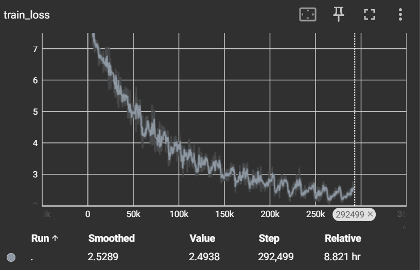
Okay, Let’s see the result. I trained the model for 20 epochs. Below are three validation examples (source, target, and model prediction).
Example 1
| Source | Block deals are usually bad news for stock prices because large-scale supplies are released to the market. |
| Target | 통상 블록딜은 시장에 대규모의 물량이 풀리는 것이어서 주가에는 악재다. |
| Predicted | ▁블록 딜 은 ▁일반적으로 ▁대규모 ▁공급이 ▁시중에 ▁풀 어서 ▁주가에 ▁대한 ▁악재가 ▁더해 지고 ▁있다 . |
Example 2
| Source | U.S. computer company Dell collaborated with actor Nikki Reed, to release the fashion brand By You with Love that recycles scrap metal from the fashion. |
| Target | 미국의 컴퓨터회사 델이 영화배우 니키 리드와 협업해 올 초 출시한 패션 브랜드 바이유위드러브는 폐금속을 재활용한다. |
| Predicted | ▁미국 ▁컴퓨터 ▁기업 ▁델 이 ▁배우 ▁니키 ▁러 프와 ▁협업 하며 ▁패션 ▁브랜드 ▁쪽 과 ▁금속 을 ▁제거 한 ▁사랑 으로 ▁보는 ▁패션 ▁브랜드를 ▁출시한다 . |
Example 3
| Source | In addition, the opponent team won the game by quickly noticing from ‘To My Boyfriend’ by Fin.K.L to ‘Cheap Coffee’ by Jang Gi-ha and the Faces. |
| Target | 그뿐 아니라 상대팀이 내는 핑클의 ‘내 남자 친구에게’부터 장기하와 얼굴들 ‘싸구려 커피’까지 빠르게 눈치채며 팀을 우승으로 이끌었다. |
| Predicted | ▁나아가 ▁상대 ▁팀이 ▁ ’ 나의 ▁친구 ’ 부터 ▁ ’ 내 녀 에게 ▁꼭 ▁먹어 요 ’ , ▁장기 하와 ▁함께 ▁하는 ▁ ’ 힘 들 티 ’ 까지 ▁빠르게 ▁풀 며 ▁경기를 ▁이겼다 . |
The ▁ in the predictions is the special character used by the BPE tokenizer to mark a space or word boundary. When the tokenizer decodes the model output back to text, it leaves this symbol in place instead of converting it to an actual space, so the raw decoded string looks like that. In a production pipeline you would typically post-process the decoded text to replace ▁ with a normal space.
Even though the translations are far from perfect, the results are still quite impressive. The model was trained on only about 130K sentence pairs for 20 epochs, which took roughly 9 hours on a single GPU.
Vaswani, A., et al. (2017). Attention is all you need. In Advances in Neural Information Processing Systems (Vol. 30). https://arxiv.org/abs/1706.03762 ↩︎
hkproj/pytorch-transformer. (n.d.). Attention is all you need implementation. GitHub. https://github.com/hkproj/pytorch-transformer ↩︎
Kazemnejad, A. (n.d.). Transformer architecture: The positional encoding. https://kazemnejad.com/blog/transformer_architecture_positional_encoding/ ↩︎
Ba, J. L., Kiros, J. R., & Hinton, G. E. (2016). Layer normalization. arXiv preprint arXiv:1607.06450. ↩︎
Glorot, X., & Bengio, Y. (2010). Understanding the difficulty of training deep feedforward neural networks. In Proceedings of the Thirteenth International Conference on Artificial Intelligence and Statistics (pp. 249–256). ↩︎
Sennrich, R., Haddow, B., & Birch, A. (2016). Neural machine translation of rare words with subword units. In Proceedings of the 54th Annual Meeting of the ACL (pp. 1715–1725). ↩︎
Szegedy, C., et al. (2016). Rethinking the Inception architecture for computer vision. In Proceedings of the IEEE Conference on Computer Vision and Pattern Recognition (pp. 2818–2826). ↩︎