Introduction
I’ve always been eager to dive into the fundamentals of robotics, and I finally have the opportunity through my “Autonomous Mobile Robot” course. I decided to write this blog post not only to solidify what I’ve learned but also to create a practical reference for my future work.
This post focuses on the essential keywords of autonomous systems: Perception, Navigation, Localization, Planning, and SLAM.
At its core, an “autonomous robot” is defined by its ability to:
- Map the World: Build or maintain a model of the environment.
- See and Understand: Perceive and analyze its surroundings.
- Know Its Place: Identify its own location and state within the map.
- Act Strategically: Plan and execute movements to navigate effectively.
Spatial Descriptions and Transformations
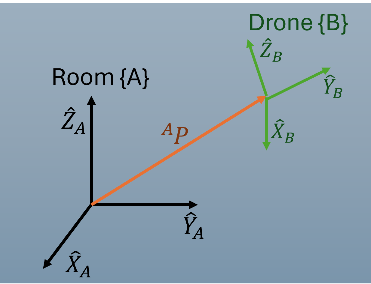
In Figure 1, {A} represents the room and {B} represents the drone. (As you can see, the drone is slightly tilted.) Why is it essential to define both a Local Coordinate System {B} and a Global Coordinate System {A} for a robot?
1. Why do we need a Local Frame {B}?
It simplifies the description of the robot’s internal structure. By using {B}, the positions of the robot’s parts (e.g., propellers, sensors, or limbs) remain constant, avoiding the need to re-calculate every minor movement relative to the entire room.
2. Why must we then express {B} in terms of {A}?
It provides the spatial context for Global Localization. A robot cannot navigate to a specific target (e.g., $x=5, y=3$) unless it knows its own position and orientation (heading) relative to the fixed world frame {A}.
SLAM (Simultaneous Localization and Mapping) is the process of a robot autonomously discovering the transformation between these two frames, allowing it to understand its body’s movement ({B}) within the context of the wider world ({A}).
Position
To know the drone’s position, we should know $^A P$. $$^A P= \begin{bmatrix} P_x \\ P_y \\ P_z \end{bmatrix}$$
So, $^A P$ is simply a position of drone relative to {A}. Then how can we calculate $^A P$? maybe by GPS, external camera system, or Odometry.
Orientation
To define the drone’s orientation (heading), we use the Rotation Matrix $^A_B R$. This matrix represents the orientation of the local frame $\{B\}$ relative to the global frame $\{A\}$: $$^A_B R = \begin{bmatrix} ^A \hat{X}_B, ^A \hat{Y}_B, ^A \hat{Z}_B \end{bmatrix}$$
- $^A \hat{X}_B$ is the unit vector representing the x-axis of $\{B\}$ expressed in the coordinate system of $\{A\}$.
- $^A \hat{Y}_B$ and $^A \hat{Z}_B$ similarly represent the y and z axes of the drone relative to the room.
Then how can we estimate $^A_B R$ in practice? We need to implement methods to compute the rotation matrix using sensor data, such as IMU readings or visual odometry from camera feeds.
For example, let $\hat{X}$ be the direction the robot is facing, $\hat{Y}$ the direction of its left arm, and $\hat{Z}$ the direction of its head. If $^A_B R$ is given as: $$^A_B R= \begin{bmatrix} 1&0&0 \\ 0&0&-1 \\ 0&1&0 \end{bmatrix}$$
This implies that:
- The robot’s face ($\hat{X}_B$) is still aligned with the world’s $+X_A$ direction $(1, 0, 0)$.
- The robot’s left arm ($\hat{Y}_B$) is now pointing towards the world’s $+Z_A$ direction $(0, 0, 1)$.
- The robot’s head ($\hat{Z}_B$) is pointing towards the world’s $-Y_A$ direction $(0, -1, 0)$.
Suppose we have detected that the robot has rotated $30^\circ$ counter-clockwise (CCW) using its onboard sensors. Now, our goal is to build a mathematical “Translator (Rotation Matrix)” that maps everything from the robot’s perspective $\{B\}$ to the room’s global frame $\{A\}$.
The most fundamental way to build this matrix in 3D is through the Dot Product. By definition, the dot product of two unit vectors represents the projection of one axis onto another. It tells us: “How much of the robot’s axis aligns with the room’s axis?”
The Rotation Matrix is composed of nine entries, where each column represents one of the robot’s axes ($\hat{X}_B, \hat{Y}_B, \hat{Z}_B$) projected onto the room’s global axes ($\hat{X}_A, \hat{Y}_A, \hat{Z}_A$):
$$^A_B R = \begin{bmatrix} \hat{X}_A \cdot \hat{X}_B & \hat{X}_A \cdot \hat{Y}_B & \hat{X}_A \cdot \hat{Z}_B \\ \hat{Y}_A \cdot \hat{X}_B & \hat{Y}_A \cdot \hat{Y}_B & \hat{Y}_A \cdot \hat{Z}_B \\ \hat{Z}_A \cdot \hat{X}_B & \hat{Z}_A \cdot \hat{Y}_B & \hat{Z}_A \cdot \hat{Z}_B \end{bmatrix}$$
- Column 1 ($^A \hat{X}_B$): Represents the robot’s “Forward” direction in the room.
- Column 2 ($^A \hat{Y}_B$): Represents the robot’s “Left” direction in the room.
- Column 3 ($^A \hat{Z}_B$): Represents the robot’s “Up” direction in the room.
3.The true power of this matrix lies in its ability to transform raw sensor data into global coordinates. Even if the drone is tilted or rotating, we can instantly calculate the global position of any detected object.
If the drone’s sensors detect a wall at a local coordinate of $^B P_{wall} = [2, 0, 1]^T$ (2m ahead and 1m above the drone), its absolute position in the room ${A}$ is:
$$\text{Wall Position in } A = \ ^A P_{drone} + \ ^A_B R \cdot \begin{bmatrix} 2 \\ 0 \\ 1 \end{bmatrix}$$
By using this Projection-based Matrix, the robot no longer sees just a wall in front of me. it understands exactly where that wall exists in the world.
First, let’s say the robot didn’t move and didn’t rotate at all. then, $$^A P_{drone} = \begin{bmatrix} 0 \\ 0 \\ 0 \end{bmatrix}, ^A_B R = \begin{bmatrix} 1 & 0 & 0 \\ 0 & 1 & 0 \\ 0 & 0 & 1 \end{bmatrix}$$
$$\text{Wall Position in } A = \begin{bmatrix} 0 \\ 0 \\ 0 \end{bmatrix} + \begin{bmatrix} 1 & 0 & 0 \\ 0 & 1 & 0 \\ 0 & 0 & 1 \end{bmatrix} \begin{bmatrix} 2 \\ 0 \\ 1 \end{bmatrix}$$ $$= \begin{bmatrix} 2 \\ 0 \\ 1 \end{bmatrix}$$
Now, let’s say the robot didn’t move, but rotated $30^\circ$ counter-clockwise (CCW) around the global Z-axis.
Even if the robot stays at the origin ($^A P_{drone} = [0,0,0]^T$), its local axes ($\hat{X}_B, \hat{Y}_B, \hat{Z}_B$) are no longer aligned with the room’s axes. To build the new Rotation Matrix, we calculate the Dot Product for each entry to see how the robot’s new directions project onto the room.
(Following the right-hand rule, a counter-clockwise (CCW) rotation is defined as a positive angle. Therefore, we substitute $\theta = +30^\circ$ into our trigonometric functions to calculate the entries of the rotation matrix.)
For the robot’s Forward direction ($\hat{X}_B$):
- $\hat{X}_A \cdot \hat{X}_B = \cos(30^\circ) \approx 0.866$
- $\hat{Y}_A \cdot \hat{X}_B = \sin(30^\circ) = 0.5$
- $\hat{Z}_A \cdot \hat{X}_B = 0$ (No vertical tilt)
For the robot’s Left direction ($\hat{Y}_B$):
- $\hat{X}_A \cdot \hat{Y}_B = \cos(90^\circ+30^\circ) = -\sin(30^\circ) = -0.5$
- $\hat{Y}_A \cdot \hat{Y}_B = \cos(30^\circ) \approx 0.866$
- $\hat{Z}_A \cdot \hat{Y}_B = 0$
For the robot’s Up direction ($\hat{Z}_B$):
- Since it rotated around the Z-axis, $\hat{Z}_B$ is still $[0, 0, 1]^T$ relative to $\{A\}$.
$$^A_B R = \begin{bmatrix} 0.866 & -0.5 & 0 \\ 0.5 & 0.866 & 0 \\ 0 & 0 & 1 \end{bmatrix}$$
Now, we apply this to the same wall detection ($^B P_{wall} = [2, 0, 1]^T$):
$$\text{Wall Position in } A = \begin{bmatrix} 0 \\ 0 \\ 0 \end{bmatrix} + \begin{bmatrix} 0.866 & -0.5 & 0 \\ 0.5 & 0.866 & 0 \\ 0 & 0 & 1 \end{bmatrix} \begin{bmatrix} 2 \\ 0 \\ 1 \end{bmatrix}$$
$$= \begin{bmatrix} (0.866 \times 2) + (-0.5 \times 0) + (0 \times 1) \\ (0.5 \times 2) + (0.866 \times 0) + (0 \times 1) \\ (0 \times 2) + (0 \times 0) + (1 \times 1) \end{bmatrix} = \begin{bmatrix} 1.732 \\ 1.0 \\ 1.0 \end{bmatrix}$$
Also, as you can see, every column of $^A_B R$ is orthogonal, which means $^A_B R$ is orthogonal matrix. So, $^A_B R^{-1}=$ $^B_A R =$ $^A_B R^T$
Frame
What is Frame? : A set of four vectors giving position and orientation information
Frame {B} = $^A \hat{X}_B$ $^A \hat{Y}_B$ $^A \hat{Z}_B$ $^A P_{BORG}$
Homogeneous Transform
As discussed in the previous section, the position of an object (e.g., a wall) relative to the global frame ${A}$ can be calculated by combining translation and rotation: $$^A P_{wall} = \ ^A P_{drone} + \ ^A_B R \ ^B P_{wall}$$
While this equation is intuitive, handling translation and rotation separately can become computationally tedious, especially when dealing with multiple coordinate transformations. To simplify this, we can encapsulate both operations into a single matrix called the Homogeneous Transformation Matrix ($T$).
By augmenting our vectors with an extra dimension (using homogeneous coordinates), we can perform the same transformation with a single matrix multiplication:
$$\begin{bmatrix} ^A P_{wall} \\ 1 \end{bmatrix} = \begin{bmatrix} ^A_B R & ^A P_{drone} \\ 0 \ 0 \ 0 & 1 \end{bmatrix} \begin{bmatrix} ^B P_{wall} \\ 1 \end{bmatrix}$$
$$\underset{(4 \times 1)}{^A \bar{P}_{wall}} = \underset{(4 \times 4)}{^A_B T} \cdot \underset{(4 \times 1)}{^B \bar{P}_{wall}}$$ This approach allows us to treat a complex sequence of movements as a chain of simple matrix multiplications, which is the standard way to handle kinematics in robotics.
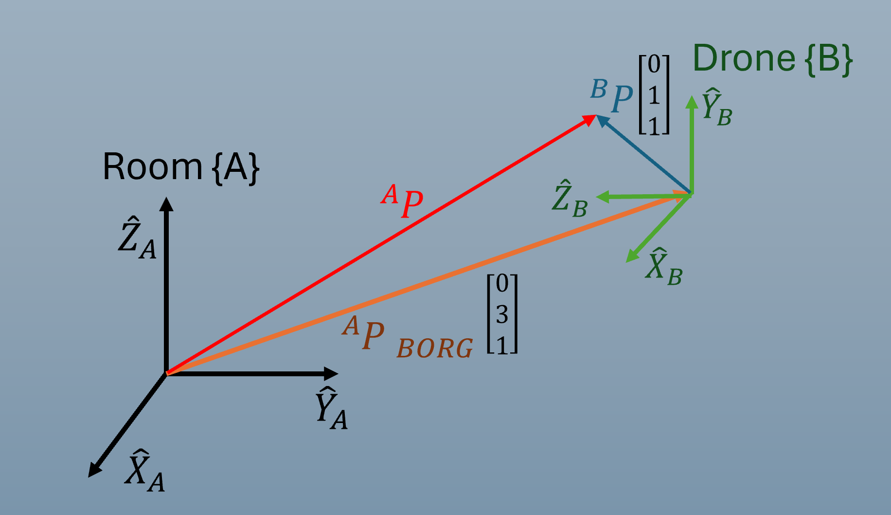
$$^A_B T = \begin{bmatrix} 1 & 0 & 0 & 0 \\ 0 & 0 & -1 & 3 \\ 0 & 1 & 0 & 1 \\ 0 & 0 & 0 & 1 \end{bmatrix}, \ ^B P=\begin{bmatrix} 0 \\ 1 \\ 1 \\ 1 \end{bmatrix}$$
$$ \ ^A P = \ ^A_B T \ ^B P \Rightarrow \ ^A P = \begin{bmatrix} 0 \\ 2 \\ 2 \\ 1 \end{bmatrix}$$
Inverse Transform
Rotation matrices are orthogonal, meaning $R^{-1} = R^T$. However, for the Homogeneous Transformation matrix, $T^{-1} \neq T^T$.
To find the inverse transform $^B_A T$ (which maps a point from frame ${A}$ back to ${B}$), we use the following structure:
If we have:$$^A_B T = \begin{bmatrix} ^A_B R & ^A P_{BORG} \\ 0 \ 0 \ 0 & 1 \end{bmatrix}$$Then its inverse $^B_A T$ is calculated as:$$^B_A T = (^A_B T)^{-1} = \begin{bmatrix} (^A_B R)^T & - (^A_B R)^T \ ^A P_{BORG} \\ 0 \ 0 \ 0 & 1 \end{bmatrix}$$Since $(^A_B R)^T = \ ^B_A R$, we can also write it as:$$^B_A T = \begin{bmatrix} ^B_A R & - ^B_A R \ ^A P_{BORG} \\ 0 \ 0 \ 0 & 1 \end{bmatrix}$$
*$- ^B_A R \ ^A P_{BORG} = \ ^B P_{AORG}$
$$ ^A_B T \ ^B_C T \ ^C_D T \ ^D_A T = I $$ $$ ^B_A T = \ ^B_C T \ ^C_D T \ ^D_A T $$
Filter
Why filter is necessary?
When a robot tries to figure out where it is (Localization), it usually relies on two main methods. However, both have critical flaws.
- Odometry (Wheel Encoders): “I turned the wheels 10 times, so I must have moved 1 meter.” This is a guess based on movement. If the wheels slip or the ground is uneven, errors accumulate over time, and the robot eventually gets lost.
- External Sensors (GPS, LiDAR, Camera): These tell the robot its current position directly, but they are full of noise (uncertainty). GPS might have an error of several meters, and LiDAR can give erratic readings when hitting reflective surfaces like glass.
Since both “Internal Prediction” and “External Observation” are never 100% accurate, we need a mathematical way to blend them to calculate the most probable state. This is the essence of a filter.
Kalman Filter
The most standard approach, which assumes that all data errors follow a Normal Distribution.
It calculates the position as “The robot is likely at this point (Mean), and the margin of error is the much (Variance).” Kalman filter is mathematically efficient and requires very little computational power, making it ideal for real-time systems. However, Accuracy drops if the robot’s movement is highly complex (Non-linear) or if the noise doesn’t follow a normal distribution. This is why variants like EKF(Extended Kalman Filter) or UKF(Unscented Kalman Filter) are often used.
Kalman filter has two steps: Prediction and Update.
Prediction (Prior)
Using the odometry data, the robot estimates its own position and velocity.
1. State Prediction $$ \hat{x}^-_k = A \hat{x}_{k-1} + B u_{k} $$
Predicts the currents state($\hat{x}_k$) based on the previous state($\hat{x}_{k-1}$) and the control input($u_k$).
A is the state transition matrix, which represents how the state changes from one time step to the next without any control input. It captures the natural physics of the system. For a robot moving at a constant velocity, $A$ would update the position based on that velocity. In our 1D example, $A=1$ means “if I don’t move, I stay where I am.”
B is the control input matrix, which defines how the control input ($u_k$), like pushing the gas pedal or turning a motor, changes the state It translates human/AI commands into physical displacement. If $u_k$ is the motor’s power, $B$ would be the coefficient that converts that power into meters moved.
2. Error Covariance Prediction $$ P^-_k = A P_{k-1} A^T + Q $$
Q (Process Noise) accounts for unmodeled factors like wind or uneven terrain. Because the world isn’t perfect, our uncertainty ($P$) always grows during this phase.
Let’s imagine a robot on a 1D linear track. It believes it is at 10m ($\hat{x}_{k-1}=10$) with 2m of uncertainty ($P_{k-1}=2$).
Prediction : Using our physics model ($A=1$, $B=1$), the robot predicts it is now at 15m ($\hat{x}^-_k=10+5=15$).
Uncertainty Growth: Due to motor noise ($Q=1$), the uncertainty grows to 3 ($P_{k}^-=3$).
Update (Posterior)
Using the external sensor data, the filter corrects the position estimate.
1. Kalman Gain $$K_k = \frac{P_k^- H^T}{HP_k^- H^T + R}$$
The Kalman Gain ($K$) acts as a relative weight that balances the prediction error covariance ($P_k^-$) against the measurement noise covariance ($R$).
H is the observation matrix, which maps the true space into the observed sensor space. Sometimes sensors don’t measure what we want directly. For example, if our state is “Position” but the sensor measures “Voltage,” $H$ acts as the bridge/converter between them.
- When $P$ is large (High Prediction Error): $K$ approaches 1. The filter “distrusts” the internal model and relies almost entirely on the sensor ($z_k$).
- When $R$ is large (High Sensor Noise): $K$ approaches 0. The filter “ignores” the noisy sensor and sticks to its internal physics-based prediction.
2. State Update $$\hat{x}_k = \hat{x}_k^- + K_k(z_k - H\hat{x}_k^-)$$
We take our guess and add a correction based on the Innovation (the difference between the sensor reading $z_k$ and our prediction).
3. Error Covariance Update $$P_k = (I - K_k H)P_k^-$$
Since we combined two sources of information, our final uncertainty ($P$) shrinks, making the estimate more precise than either source alone.
A GPS sensor (error variance $R=2$) reports the robot is at 18m ($z_k=18$).
Kalman Gain: $$ K_k = \frac{P_k^- H^T}{HP_k^- H^T + R} = \frac{3 \times 1}{1 \times 3 + 2} = \frac{3}{5} = 0.6 $$
Since our internal uncertainty (3) is higher than the sensor noise (2), we trust the sensor more ($60%$).
State Update: $$\hat{x}_k = \hat{x}_k^- + K_k(z_k - H\hat{x}_k^-) = 15 + 0.6(18 - 15) = 16.8$$
The result is a weighted average that leans toward the sensor.
Error Covariance Update: $$P_k = (I - K_k H)P_k^- = (1 - 0.6 \times 1) \times 3 = 1.2$$
Particle Filter
While the Kalman Filter relies on Gaussian assumptions, the Particle Filter (also known as Sequential Monte Carlo) uses a simulation-based approach to estimate the state of a robot. It represents the probability distribution of the robot’s position as a set of discrete samples, or “Particles.”
Each particle $i$ consists of a state hypothesis $x_k^{(i)}$ and an associated weight $w_k^{(i)}$, which represents the probability (confidence) of that hypothesis.
1. Prediction (Sampling)
We propagate each particle forward in time using the robot’s motion model and control input $u_k$. $$x_k^{(i)} \sim p(x_k | x_{k-1}^{(i)}, u_k)$$
2. Update (Importance Weighting)
When a sensor measurement $z_k$ is received, we evaluate how “likely” each particle is by calculating its Importance Weight. $$w_k^{(i)} = w_{k-1}^{(i)} \cdot p(z_k | x_k^{(i)})$$
Likelihood ($p(z_k | x_k^{(i)})$): We compare the sensor data to what the particle should see at its current location. Particles that match the sensor data closely receive high weights; those that don’t are penalized with low weights.
3. Resampling
To prevent particles with low weights from dominating the estimate, we “resample” the particles based on their weights. High-weight particles are duplicated, while low-weight particles are discarded.
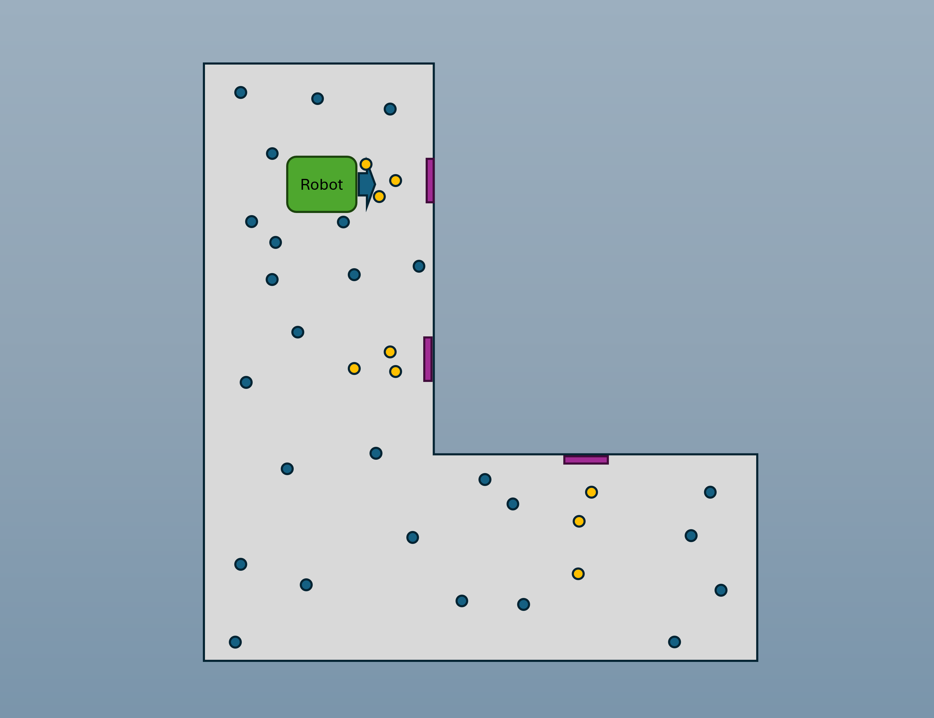
Let’s imagine that the robot is provided with a pre-installed map ($m$), but its initial pose ($x_0$) is completely unknown. To solve this, the robot uses a Particle Filter to recursively estimate its position.
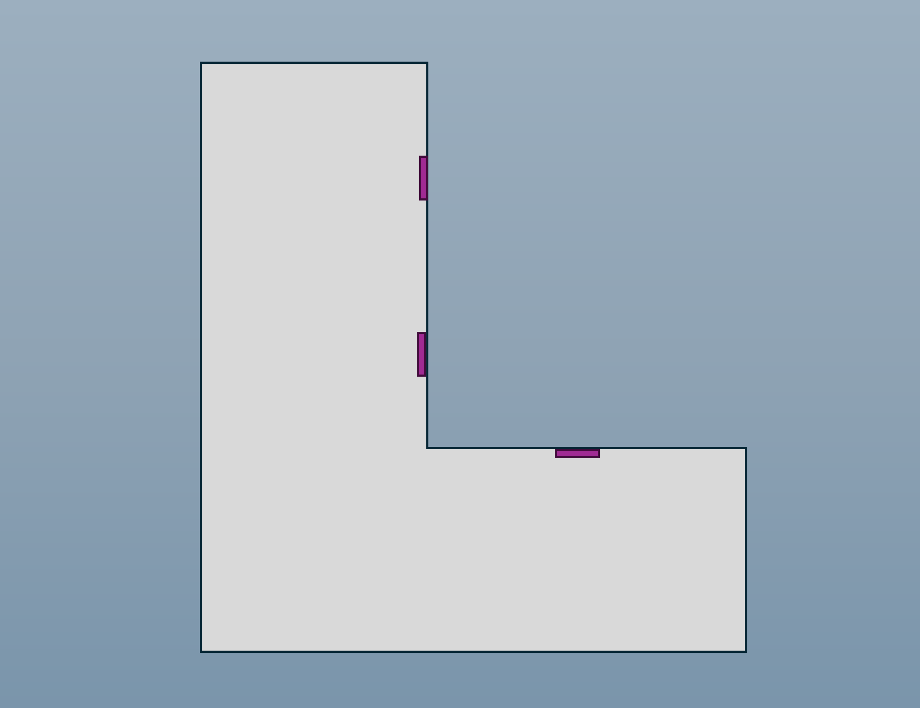
Since the robot has no prior knowledge of its coordinates, it initializes $N$ particles ${x_0^{(i)}, w_0^{(i)}} \ _{i=1}^N$ typically distributed according to a uniform prior across the map’s free space. At this stage, each particle represents a possible state of the system with an equal weight of $N^{-1}$.
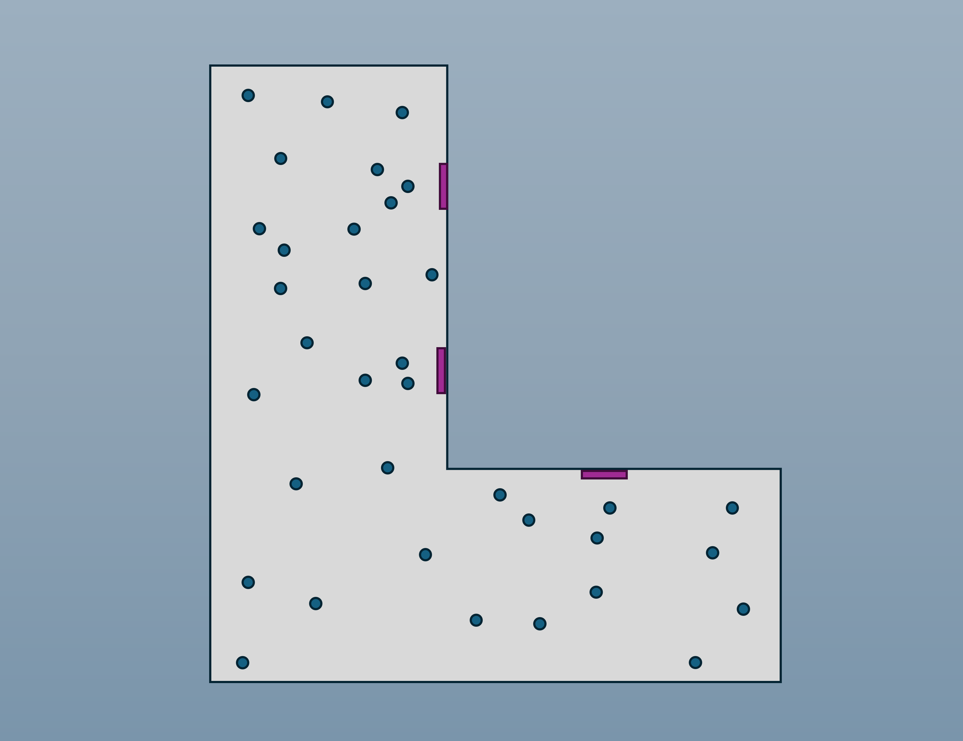
The robot’s camera, pointed at the right-side wall, captures a purple door. This triggers the Measurement Update phase.
- Weight Update (Importance Weighting): For every particle, we calculate the Likelihood. “Given this particle’s hypothesized location, what is the probability of seeing a purple door?”
- Numerical Calculation: We use a Gaussian Probability Density Function (PDF) to score the particles: $$w_k^{(i)} = \eta \cdot p(z_k | x_k^{(i)}, m)$$
where $z_k$ is the actual measurement and $p(z_k | x_k^{(i)}, m)$ is the likelihood based on the map. Particles located in front of any of the three purple doors match the map. Their weights stay high, while particles in front of plain walls see a massive drop in weight.
After the update, most particles have negligible weights, leading to degeneracy. To fix this, the robot performs Resampling. Particles with higher weights are more likely to be selected and multiplied, while low-weight particles are eliminated.
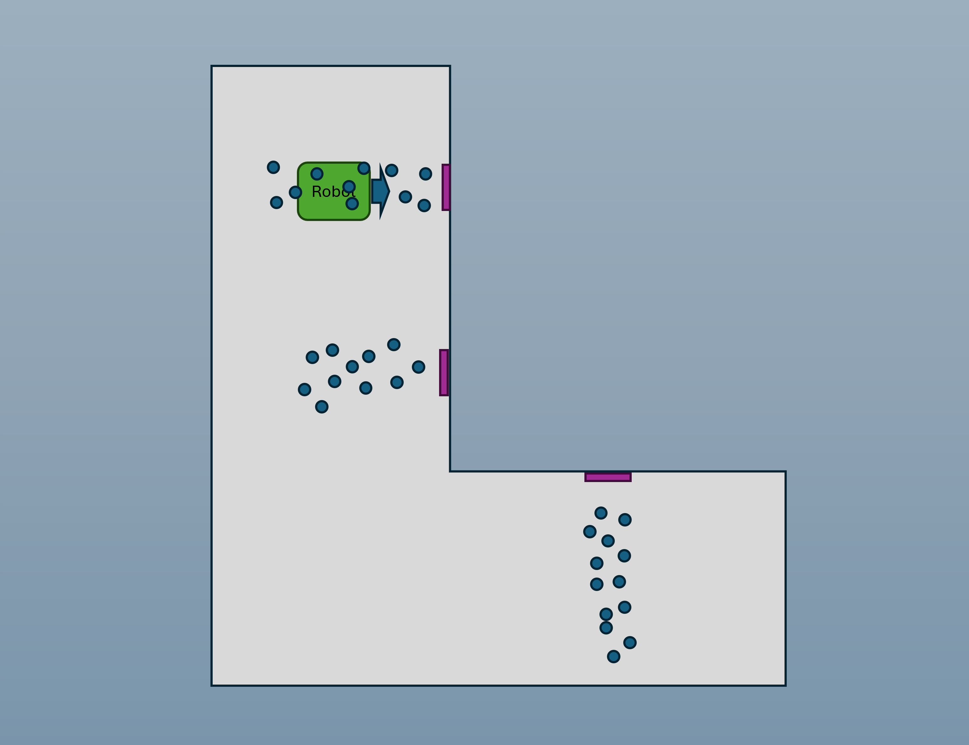
The particles now cluster into three distinct groups, one in front of each purple door on the map. This is a multi-modal distribution, representing three high-probability hypotheses.
The robot now drives forward ($u_k$). This triggers the Time Update (Prediction) phase. In a particle filter, each particle $i$ possesses its own state $x_k^{(i)} = [x, y, \theta]^T$, where $\theta$ represents its orientation. When the “move forward” command is issued, every particle projects its position based on its own heading ($\theta$):
We add process noise ($Q$) to account for uncertainties like wheel slip or mechanical errors.
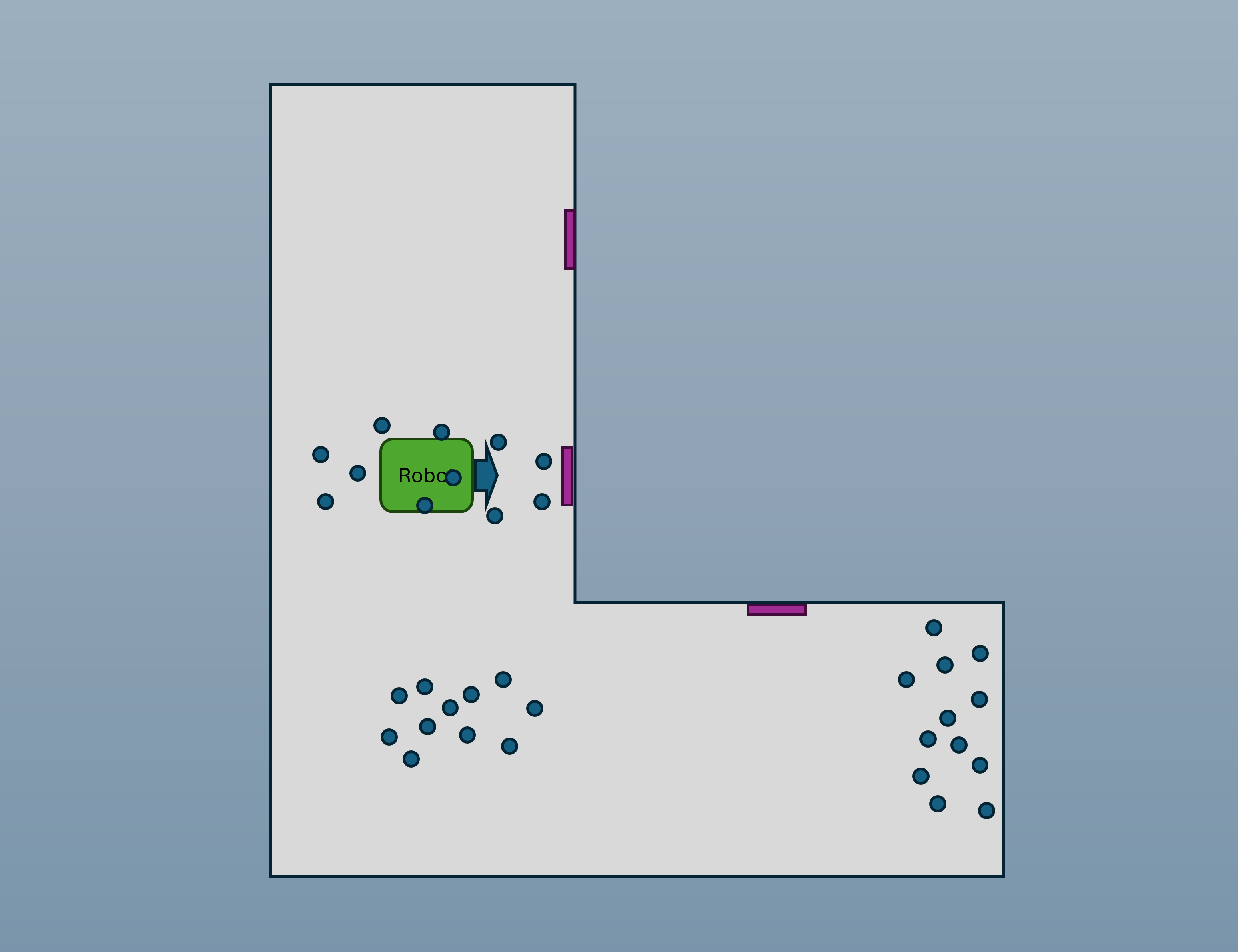
As the robot moves, the camera captures a second purple door. This is the deciding moment for our hypotheses.
Hypothesis A : These particles were correctly facing downward at the first door. Upon receiving the “forward” command, they moved down along the corridor to the second door. Their predicted measurement ($\hat{z}$) from the map perfectly matches the actual measurement ($z_k$) of the purple door. Consequently, their likelihood $p(z_k | x_k^{(i)}, m)$ is maximized, and they will flourish during resampling.
Hypothesis B : These particles also faced downward but started at the second door. After moving forward, they are now in the open space at the bottom of the L-shape. According to the map, their right-side camera should see a distant wall or empty space. Since the sensor sees a door, the mismatch causes their likelihood to drop to near zero.
Hypothesis C : These particles were located at the third door but were facing rightward to see the door initially. When the robot commanded a “forward” move, these particles traveled toward the right wall of the map. Furthermore, because they are facing right, their right-side camera is now looking at the upper wall of the corridor. This total contradiction between their predicted view and the actual purple door seen by the robot results in their immediate elimination during Resampling.
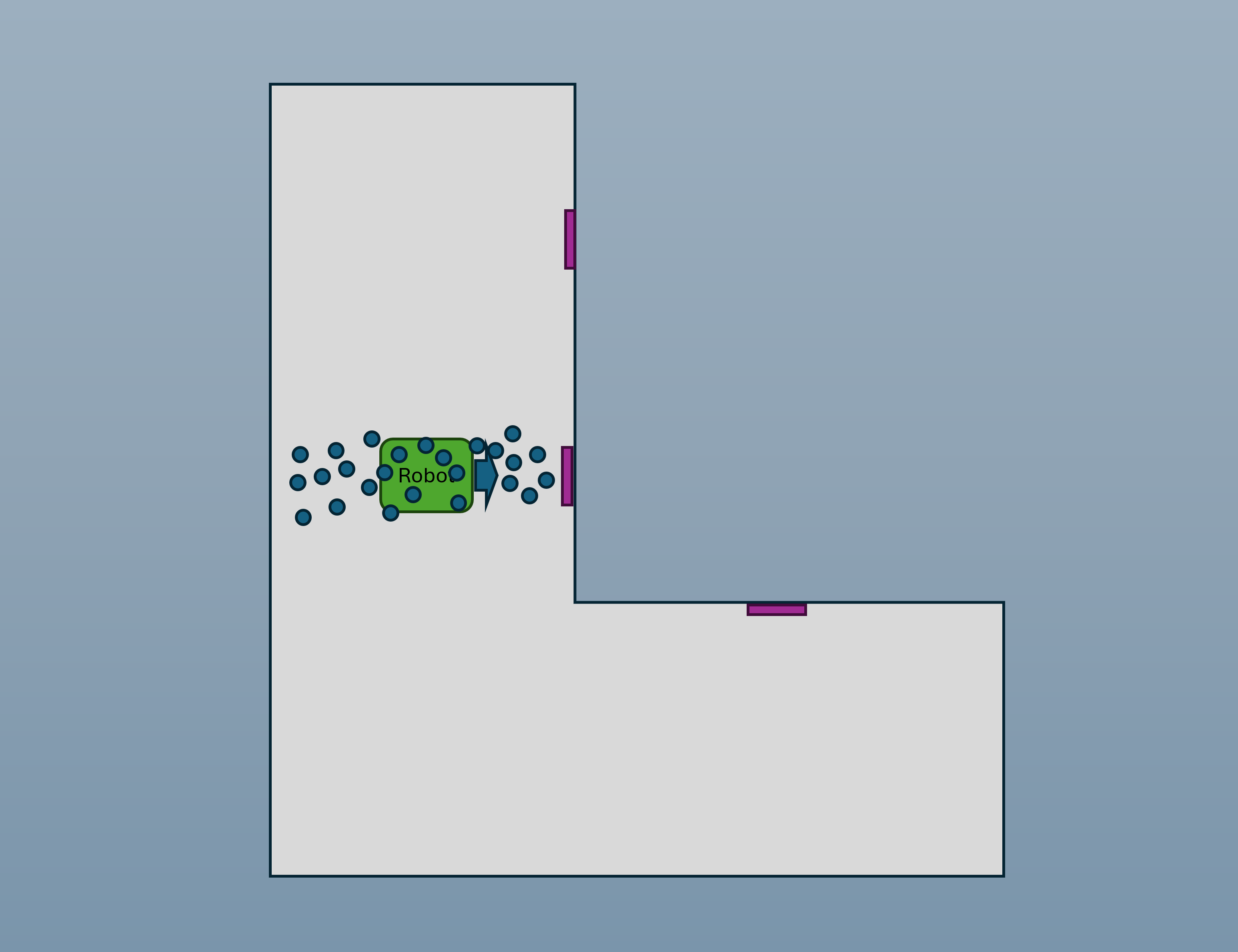
After the resampling, all 1,000 particles collapse into a single, tight cluster in front of the second purple door. The robot has successfully localized itself by mathematically proving that only one starting position is consistent with the sequence of observations.
Graph
In the previous chapter, we used Filters (Kalman Filter and Particle Filter) to answer the question: “Where am I?” But localization is just the beginning. To be truly autonomous, a robot must decide: “How do I get to my destination efficiently?” This is where Graph Theory comes in.
The physical world is continuous and infinitely complex, but a robot’s brain needs structure to make decisions. By abstracting the environment into a Graph $G=(V,E)$, a set of vertices (states) and edges (paths), we simplify the infinite world into a manageable mathematical map.
While filters are the robot’s eyes, Graph Theory is its intelligence. Even the most advanced autonomous systems today rely on this hierarchical approach: using Graphs for Global Planning and continuous math for local movement.
Dijkstra’s Algorithm
Dijkstra’s Algorithm is a graph search algorithm that finds the shortest path between two nodes in a graph. It is a greedy algorithm that works by iteratively selecting the node with the smallest distance from the start node.
Single Source Shortest Path Problem
Dijkstra’s algorithm is designed to solve a specific optimization problem: Given a graph with non-negative edge weights, find the shortest path from a starting node (Source) to every other node in the network.
- Objective: Minimize the total cost(distance, time, energy, etc.) of travel.
- Constraint: Edge weights must be non-negative.($w \geq 0$)
Relaxation
Relaxation is the key operation in Dijkstra’s algorithm. It updates the distance to a node if a shorter path is found.
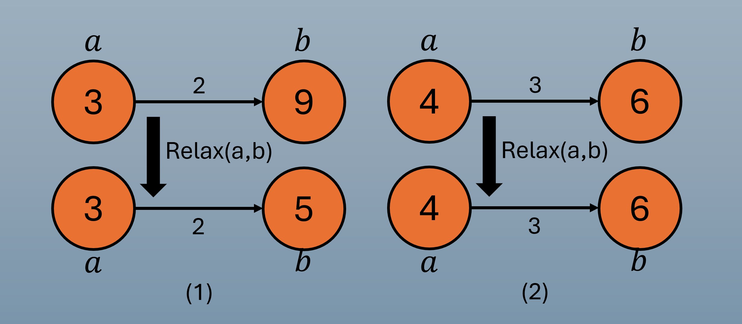
In (1), the shortest distance to node $b$ discovered so far is 9. However, we have found a new path to $b$ via node $a$ with a lower total cost of 5. Consequently, we update the shortest distance for node $b$ to 5 and set node $a$ as its new parent in the shortest path.
In (2), the shortest distance to node $b$ is already 6. Although we found an alternative path to $b$ through node $a$, its total cost is 7. Since the existing path is more efficient, we maintain the shortest distance for node $b$ at 6.
As shown in these examples, the “relaxation” step acts as a core optimization operation that constantly refines the robot’s knowledge.
def relax(a, b, G):
    if b.dist() > a.dist() + G.weight(a,b): # G is a graph object
        b.set_dist(a.dist() + G.weight(a,b)) # set the distance of node b to a.dist() + G.weight(a,b)
        b.set_parent(a) # set the parent of node b to a
Pseudo-code for Dijkstra’s Algorithm
def Dijkstra(G, s):
    # Initialization: Set up initial distances and parents
    for a in G.nodes(): # For each node a in the graph's node set
        a.set_dist(float('inf')) # Initialize distance to infinity
        a.set_parent(None)       # Initialize parent as None
    # s is also in the G.nodes()
    s.set_dist(0) # Set distance of the source node to 0
    S = set() # Set of nodes whose shortest-path weights are already determined
    Q = PriorityQueue(G.nodes()) # Priority Queue of nodes
    while not Q.is_empty():
        a = Q.pop_min()
        S.add(a) # Add a to the set of nodes whose shortest-path weights are already determined
        for b in a.adjacent_nodes():
            if b.dist > a.dist + G.weight(a, b):
                relax(a, b, G) # Relax the edge (a, b)
                Q.modify_key(b) # Reorganize the priority queue as b's distance has decreased
    return G # Return the graph with updated shortest path information
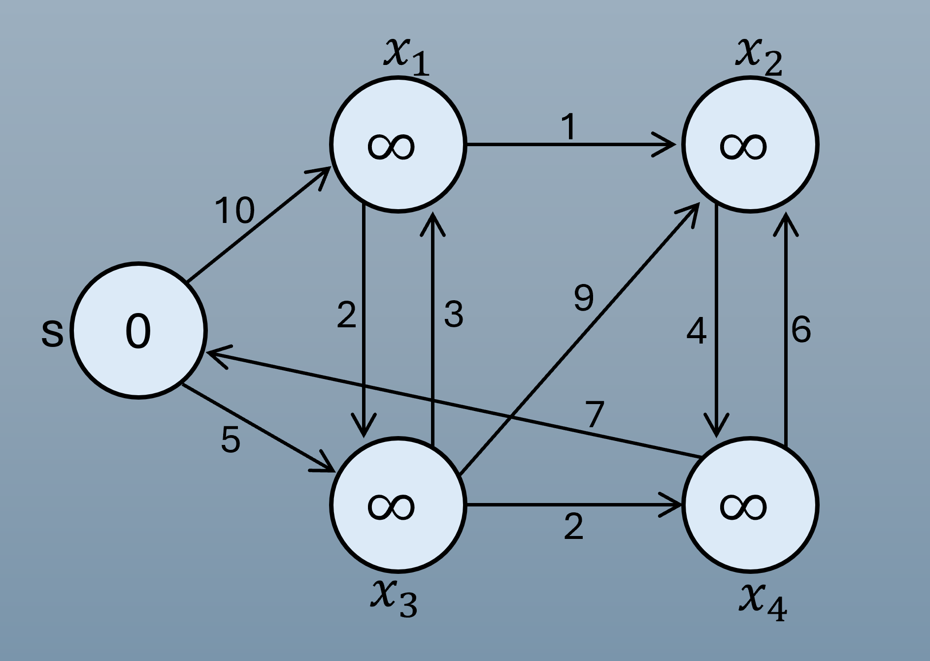
In Figure 10, $S$ is empty and $Q= \{s(0), x_1(\infty), x_2(\infty), x_3(\infty), x_4(\infty)\}$. Since Q is not empty, the while loop is executed.
First while loop. Because of Q.pop_min(), $a=s(0)$ is extracted from $Q$ and added to $S$. $S=\{s(0)\}$. And the for loop is executed.
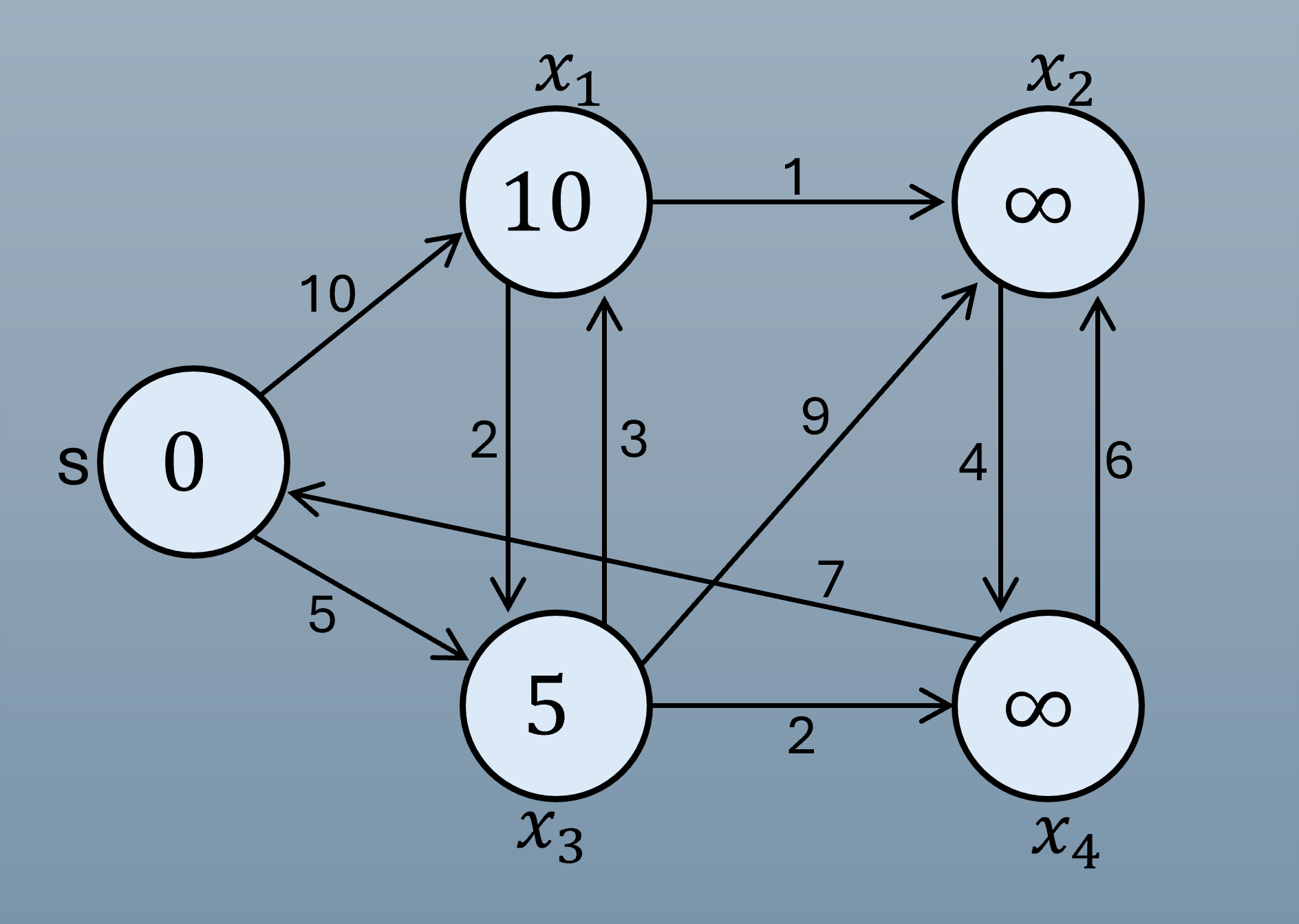
After the for loop ran one time, $Q= \{x_3(5), x_1(10), x_2(\infty), x_4(\infty)\}$. And the while loop is executed again.
Second while loop. At this time, $a=x_3(5)$ is extracted from $Q$ and added to $S$. $S=\{s(0), x_3(5)\}$. And the for loop is executed. Because this is directed graph, adjacent nodes of $x_3(5)$ are $x_1(10)$, $x_2(\infty)$, and $x_4(\infty)$.
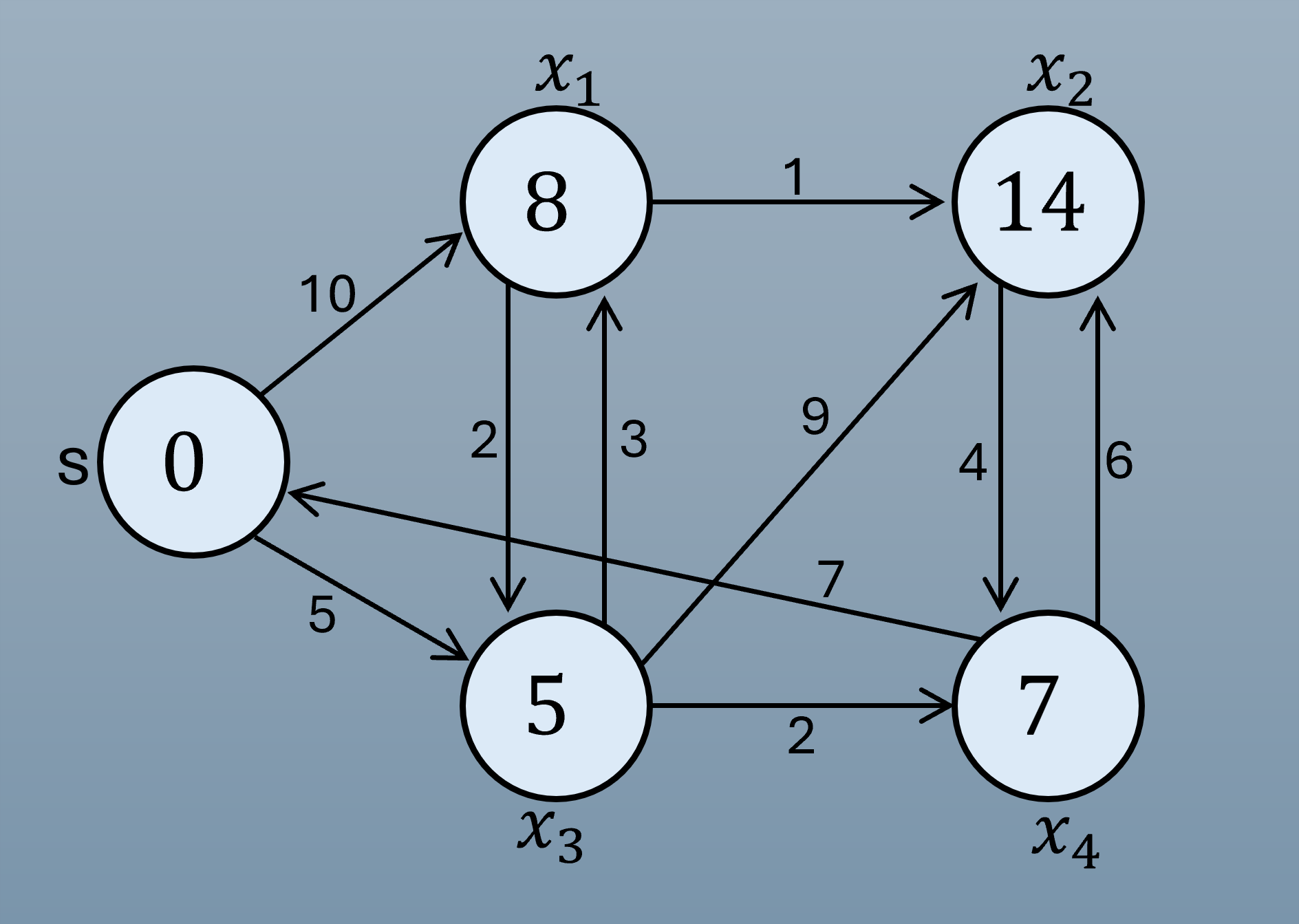
$Q= \{x_4(7), x_1(8), x_2(14)\}$. Third while loop. Next time, $x_4(7)$ is extracted from $Q$ and added to $S$. $S=\{s(0), x_3(5), x_4(7)\}$. $a$ is $x_4(7)$ and the adjacent nodes are $s$ and $x_2(14)$.
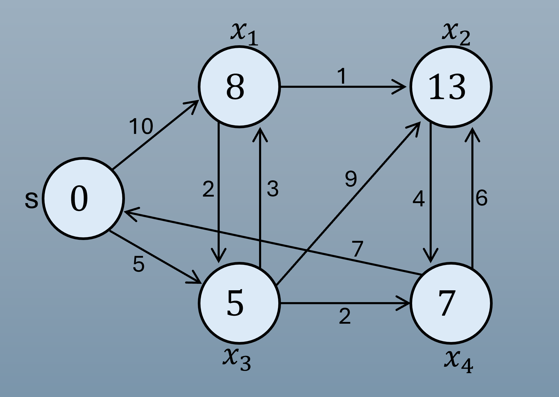
$x_2(14)$ is turned into $x_2(13)$. $Q= \{x_1(8), x_2(13)\}$. Fourth while loop. a is $x_1(8)$ and the adjacent nodes are $x_3(5)$ and $x_2(13)$. $S=\{s(0), x_3(5), x_4(7), x_1(8)\}$.
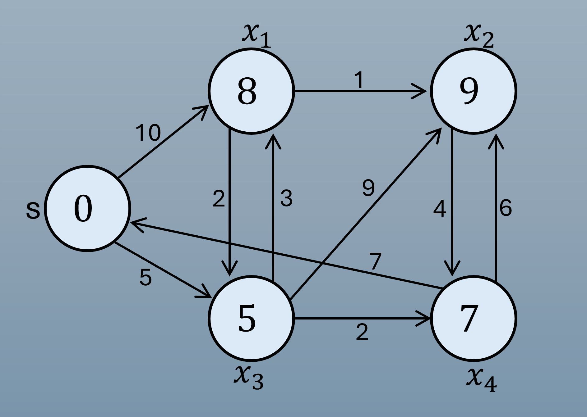
Now, $Q= \{x_2(9)\}$. Fifth while loop. a is $x_2(9)$ and the adjacent node is only $x_4(7)$. $S=\{s(0), x_3(5), x_4(7), x_1(8), x_2(9)\}$. This time, nothing happens because $x_4$’s distance(7) is already less than 9+4=13.
Understanding Time Complexity $O(n^2)$
Dijkstra’s algorithm operates in $O(n^2)$ time (where $n$ is the number of vertices) due to its nested search structure.
- 1. Outer Loop ($n$ iterations): The algorithm must extract each of the $n$ nodes from the Priority Queue exactly once to determine its final shortest path.
- 2. Inner Loop (Up to $n-1$ iterations): For each extracted node, the robot scans all its adjacent neighbors to perform Relaxation. In the worst-case scenario (a complete graph where every node is connected to every other node), each node will have $n-1$ neighbors to check.
$$n \text{ (Nodes)} \times (n-1) \text{ (Max Neighbors per Node)} = n^2 - n \approx O(n^2)$$
Kinematics
Through Filtering (Kalman/Particle Filters), the robot can now estimate its current pose despite sensor noise. Through Graph-based Path Planning (Dijkstra’s Algorithm), it can determine the most efficient route to its destination.
However, knowing where to go and where you are is not enough. A crucial question remains. How does the robot actually move its body to follow that path?
This is where Kinematics comes in. While our high-level planners output abstract commands like “move to $(x, y)$,” our hardware only understands low-level signals like “rotate the left wheel at $100\text{ RPM}$.” Kinematics is the mathematical language that translates these high-level strategies into physical motion.
Kinematics is a subfield of mechanics that deals with the motion of bodies without considering the forces that cause the motion.
Forward Kinematics
Forward kinematics is the process of calculating the robot’s overall position and orientation (often called the pose) based on known actuator positions or speeds.
- Q : “If my left wheel spins at $X$ RPM and my right wheel spins at $Y$ RPM, where will my robot be after 5 seconds?”
This is essential for Odometry, where the robot tracks its own movement over time by integrating wheel encoder data.
Inverse Kinematics
Inverse kinematics is the opposite. It starts with a desired destination or target pose and calculates the specific actuator commands needed to get there.
- Q : “I want my robot to move to coordinate $(x, y)$ with an orientation of $\theta$. How fast should each wheel spin to achieve this?”.
This is the foundation of Motion Control. When a path planner tells the robot to follow a specific trajectory, inverse kinematics translates that path into actual motor signals.
Mobile Robot kinematics
Let’s compare robot arm and mobile robot.
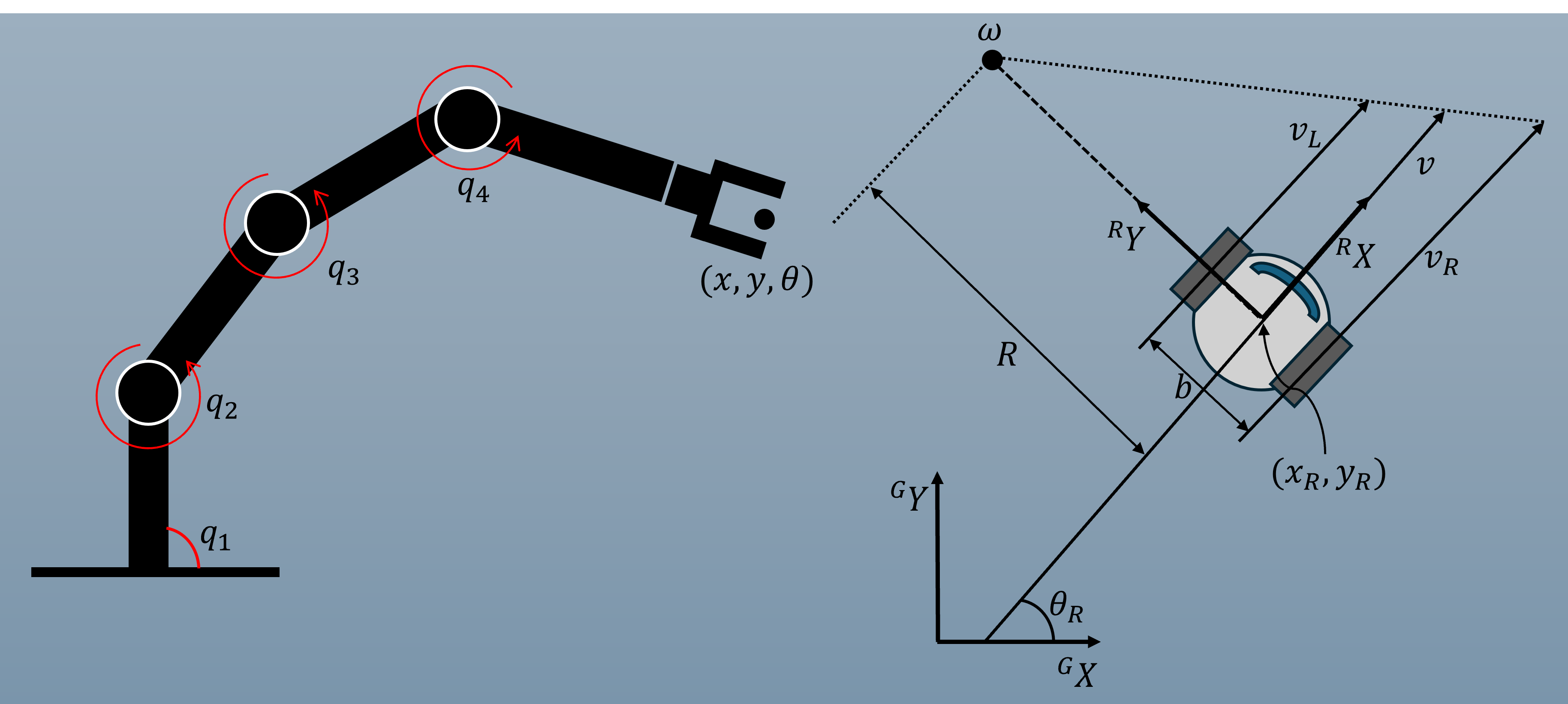
| Feature | Robot Arm | Mobile Robot |
|---|---|---|
| Input (Joint Space) | $q_1, q_2, q_3, q_4$ (Joint Angles) | $v_L, v_R$ (Left/Right Wheel Velocities) |
| End-Effector (Pose) | $x, y, \theta$ (Gripper Position/Orientation) | $x_R, y_R, \theta_R$ (Robot Center Pose) |
| Physical Parameter | Link Lengths ($l_1, l_2, \ldots$) | Wheel Radius ($r$), Track Width ($b$) |
| Forward Kinematics | Calculating Tip Pose from Joint Angles | Calculating Robot Trajectory from Wheel RPM |
| Inverse Kinematics | Finding Joint Angles to reach a Target Point | Finding Wheel Velocities to reach a Target Pose |
| Constraints | Limited by the Reach (Workspace) | Limited by Direction (Non-holonomic) |
Mobile robots present a unique set of challenges compared to fixed robotic arms.
- No Unique Mapping: For robotic arms, joint angles map directly to a specific endpoint. In mobile robots, wheel encoder values do not map to a unique pose because factors like wheel slip can occur.
- Unbound Mobility: Unlike arms fixed to a base, mobile robots move freely and “unbound” throughout their entire environment.
- No Direct Measurement: There is no instantaneous way to measure a mobile robot’s exact position (unlike an arm’s end-effector).
- Integration Errors: A robot’s position must be calculated by integrating its motion over time. Because this depends on the specific path taken, small measurement errors accumulate, leading to inaccuracies in the final position estimate.
- Kinematic Constraints: Understanding mobile motion starts with the physical constraints of the wheels—such as the fact that standard wheels can roll forward but cannot slide sideways.
Differential Drive Mobile Robot
The differential drive system is the most common and simplest drive mechanism for mobile robots. It consists of two wheels mounted on a common axis, each controlled by an independent motor.
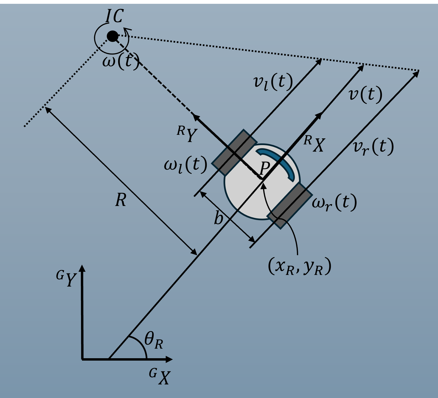
- $r$: Radius of the wheels.
- $b$: Distance between the two wheels (track width).
- $P$: The center point of the robot (midpoint of the wheel axis).
- $v_l(t), v_r(t)$: Linear velocities of the left and right wheels.
- $\omega_l(t), \omega_r(t)$: Angular velocities of the left and right wheels.
- $R$: Instantaneous curvature radius of the robot’s trajectory.
- $IC$ (or $ICC$): Instantaneous Center of Rotation.
The linear velocity of each wheel is directly proportional to its angular velocity and radius: $$v_l(t) = r \cdot \omega_l(t), \quad v_r(t) = r \cdot \omega_r(t)$$
From these, we can derive the linear velocity ($v$) and angular velocity ($\omega$) of the entire robot body:
Linear Velocity ($v$): The average speed of the two wheels.
$$v(t) = \frac{v_r(t) + v_l(t)}{2}$$Angular Velocity ($\omega$): The difference in wheel speeds divided by the track width. $$\omega(t) = \frac{v_r(t) - v_l(t)}{b}$$
Special Cases of Motion
The behavior of the robot changes significantly based on the relative velocities of the wheels:
- Straight-line Motion ($v_l = v_r$): When both wheels spin at the same speed, $\omega = 0$ and the robot moves in a straight line.
- Pure Rotation ($v_l = -v_r$): When wheels spin at the same speed in opposite directions, $v = 0$ and the robot rotates in place around its center ($P$).
- Curved Path ($v_l \neq v_r$): The robot follows a circular trajectory around the $IC$. This motion is highly sensitive to velocity errors; small deviations in wheel speed lead to different trajectories.
Kinematic Model in the Global Frame
To track the robot’s pose $[x, y, \theta]^T$ in the initial (global) frame, we integrate the velocities over time. The differential equations for the robot’s pose are: $$\dot{x}(t) = v(t) \cdot \cos\theta(t)$$ $$\dot{y}(t) = v(t) \cdot \sin\theta(t)$$ $$\dot{\theta}(t) = \omega(t)$$
The final position at time $t$ is calculated by integrating these equations:
$$\begin{cases} x(t) = \int_{0}^{t} v(\tau) \cos\theta(\tau) d\tau \\ y(t) = \int_{0}^{t} v(\tau) \sin\theta(\tau) d\tau \\ \theta(t) = \int_{0}^{t} \omega(\tau) d\tau \end{cases}$$