Introduction
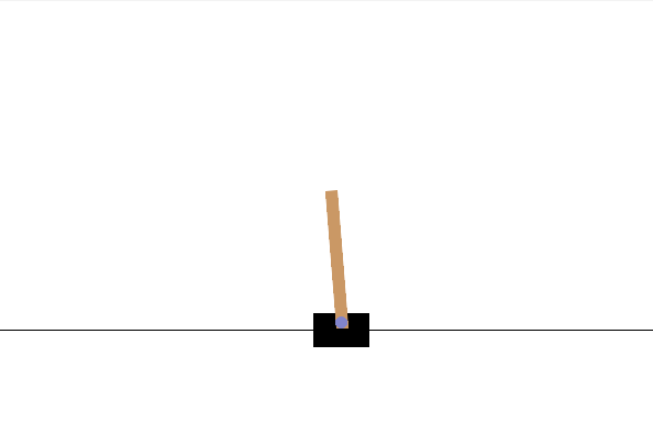
If you are interested in reinforcement learning, you have probably heard of CartPole [6], often considered the “Hello World” environment of the field. This is partly because the task is simple to understand, and partly because each episode ends quickly, allowing you to observe learning progress within a short time.
Looking back, I have run many experiments in CartPole before, but not in a structured or systematic way, which caused me to forget most of the details over time. In this post, I aim to consolidate those trials into a coherent narrative, focusing in particular on why Q-learning can become unstable and how techniques such as experience replay, Double DQN, and failure-focused sampling can improve robustness.
Full implementation code on GitHub: stabilizing-q-learning-cartpole
Experiments
1. From TD Learning to Q-Learning
Intuitively, Q-learning can be viewed as a member of the Temporal-Difference (TD) family of methods [1]. TD learning focuses on updating the value function directly, rather than optimizing the policy explicitly. We can consider $V(S_t)$ as the prediction $\hat{y}$ and $R_{t+1}+\gamma V(S_{t+1})$ as the target $y$.
This analogy to supervised learning makes the TD update in Equation (1) straightforward to implement, especially when using a neural network to approximate the value function.
#torch
env = gym.make("CartPole-v1", render_mode="none")
optimizer = torch.optim.Adam(model.parameters(), lr=0.001)
criterion = nn.MSELoss()

current_value = model(state) # V(S_t)

# (select a action to take somehow)
next_state, reward, ... = env.step(action)

next_value = model(next_state)
target_value = reward + (gamma* next_value)

criterion = nn.MSELoss()
loss = criterion(current_value, target_value)
However, the (select a action to take somehow) part is a major challenge. $V(s)$ itself doesn’t contain information about what action should be taken. If the environment were simple and deterministic, such as Chess or Go, then we could simulate all actions from $S_t$ and calculate all $V(S_{t+1})$ without actually taking those actions. With all possible $V(S_{t+1})$ values in hand, we could finally select an action by choosing the one leading to the state with the best value.
2. SARSA
That’s where the action-value function Q is effective. $V(S_t) = \max_{a}Q(S_t,a)$. Below is the SARSA algorithm [1], which leverages the action-value function Q. As you will see, we can now choose the next action without actually taking it or simulating it.
Code:
1.SARSA_cartpole.py
Click to see the SARSA torch code
model = qnetwork(4,2) # state consists of four scalars.
env = gym.make("CartPole-v1", render_mode="none")
optimizer = torch.optim.Adam(model.parameters(), lr=0.001)
criterion = nn.MSELoss()

for episode in range(3000): # 3000 episodes
    obs, info = env.reset()
    # Example output: [ 0.01234567 -0.00987654  0.02345678  0.01456789]
    # [cart_position, cart_velocity, pole_angle, pole_angular_velocity]

    game_over = False
    total_reward = 0

    action_space = [0,1] # 0: left, 1: right

    # First action of a episode should be selected here.
    state_tensor = torch.tensor(obs, dtype=torch.float32)
    q_values = model(state_tensor)
    if np.random.random() < 0.1: # epsilon = 0.1
        act = np.random.choice(action_space)
    else:
        act = torch.argmax(q_values).item()

    while not game_over:
        state_tensor = torch.tensor(obs, dtype=torch.float32)
        q_values = model(state_tensor)
        # SARSA: act is already selected. (This is the key point of SARSA.)

        # current_q is where the backpropagation starts.
        current_q = q_values[act]

        # step the environment
        next_obs, reward, terminated, truncated, info = env.step(act)
        total_reward += reward

        # SARSA: calculate the target using next_act
        with torch.no_grad(): # to block the gradient
            next_state_tensor = torch.tensor(next_obs, dtype=torch.float32)
            if np.random.random() < 0.1:
                next_act = np.random.choice(action_space)
            else:
                next_act = torch.argmax(model(next_state_tensor)).item()

            next_q = model(next_state_tensor)[next_act]
            target_q = reward + (0.99 * next_q * (1 - terminated))
            # no next reward when terminated
            # But, truncated is okay. because we can still get the next reward.

        # calculate the loss and update the model
        loss = criterion(current_q, target_q)
        #target_q here is like the label for the current_q.
        optimizer.zero_grad()
        loss.backward()
        optimizer.step()

        # SARSA: update act not only obs.
        obs = next_obs
        act = next_act  # This is the key of SARSA.
In my opinion, the main point of SARSA is to select the next action and target q-value using epsilon-greedy. (see the with torch.no_grad(): part) Let’s check the SARSA’s performance.
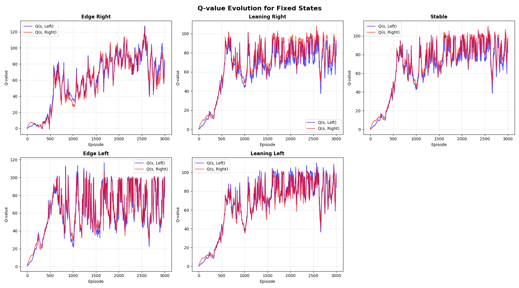
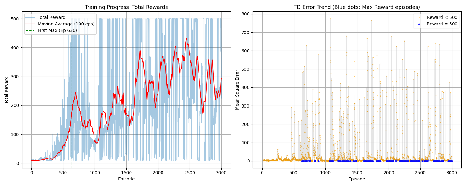
SARSA reached the maximum reward of 500, and the moving average showed an increasing trend up to a point. However, it fails to stay at the peak. What could be the reason for these periodic drops in total reward?
- FIXED EPSILON?
I fixed epsilon at 0.1, meaning that approximately every 10 steps, an action is selected randomly, and CartPole is a very sensitive environment. Even so, I believe that if the model were trained well, it should have been robust enough to handle 10% randomness.
- NN MODEL?
class qnetwork(torch.nn.Module):
    def __init__(self, state_size:4, action_size:2):
        super().__init__()
        self.fc1 = nn.Linear(state_size, 128)
        self.fc2 = nn.Linear(128, action_size)
        self.relu = nn.ReLU()

    def forward(self, x):
        x = self.relu(self.fc1(x))
        x = self.fc2(x)
        return x
Was my model not large enough or not structured well to memorize all the past information? That could be the case. Even though the training data is correlated, if the model were large enough and had many state-of-the-art features, it could memorize every past experience.
- FORGETTING?
If the problem is mainly caused by forgetting previous experiences, there could be several ways to mitigate this. Mnih et al. [2] demonstrated that leveraging Experience Replay is effective for reducing data correlation and smoothing the training distribution. Intuitively, it’s easy to see why Experience Replay can reduce data correlation—it allows us to randomly sample from several saved episodes rather than processing them consecutively. Then what does it mean that Experience Replay “smooths the training distribution?”
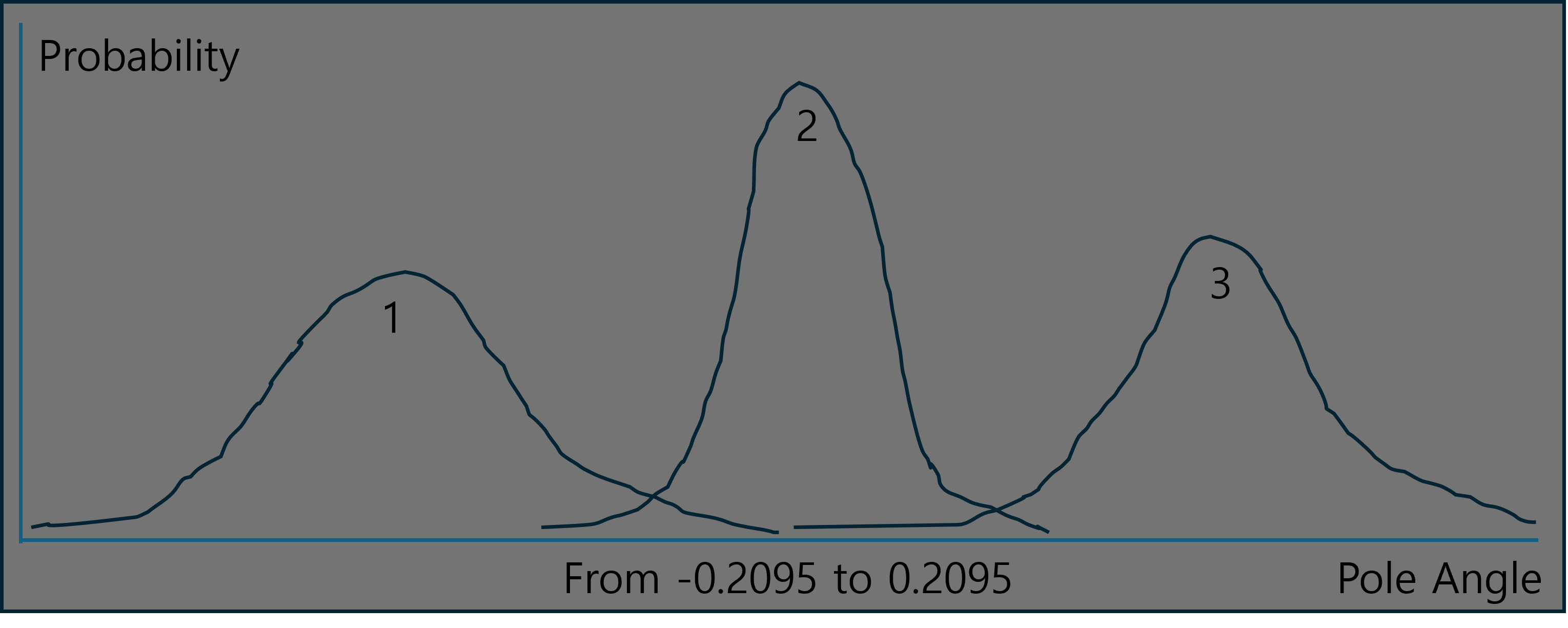
In CartPole there are four scalars in the state, but let’s think about only one scalar, Pole Angle. If training data is dominated by specific scenarios, such as left-leaning angles (Curve 1), the agent overfits and fails to handle opposite situations like right tilts. As the agent masters the task, the data distribution squeezes into a narrow curve around zero (Curve 2), causing the agent to forget recovery strategies for large deviations. (This is similar to a problem in imitation learning, which learns from expert behaviors.)
To build a robust model, the agent must learn from a comprehensive distribution that covers the entire state space. Experience Replay addresses this by randomly sampling from a diverse history of episodes. If the experience buffer successfully saves diverse scenarios, it can reconstruct a broad distribution that encompasses all scenarios.
3. Q-learning
Okay, I decided to use Experience Replay, but SARSA is incompatible with it because SARSA is an on-policy algorithm. So, it’s time to move on to Q-learning. Q-learning is an off-policy algorithm, which means we can leverage Experience Replay, and it’s similar to SARSA.
However, first, let’s look at Q-learning without Experience Replay. The main difference between Q-learning and SARSA is that when calculating the target Q, we don’t consider random actions (like in epsilon-greedy), even if the actual next action might be random—we just do exploitation. Intuitively, it makes sense to define the value of the current state based on the best possible result achievable by ideal actions from that state.
Code:
2.Qlearning_cartpole.py
        # calculate the target
        with torch.no_grad():
            next_state_tensor = torch.tensor(next_obs, dtype=torch.float32)
            next_q_max = torch.max(model(next_state_tensor))
            target_q = reward + (0.99 * next_q_max * (1 - terminated))

        loss = criterion(current_q, target_q)

        optimizer.zero_grad()
        loss.backward()
        optimizer.step()
        episode_losses.append(loss.item())

        obs = next_obs
Let’s check the results.
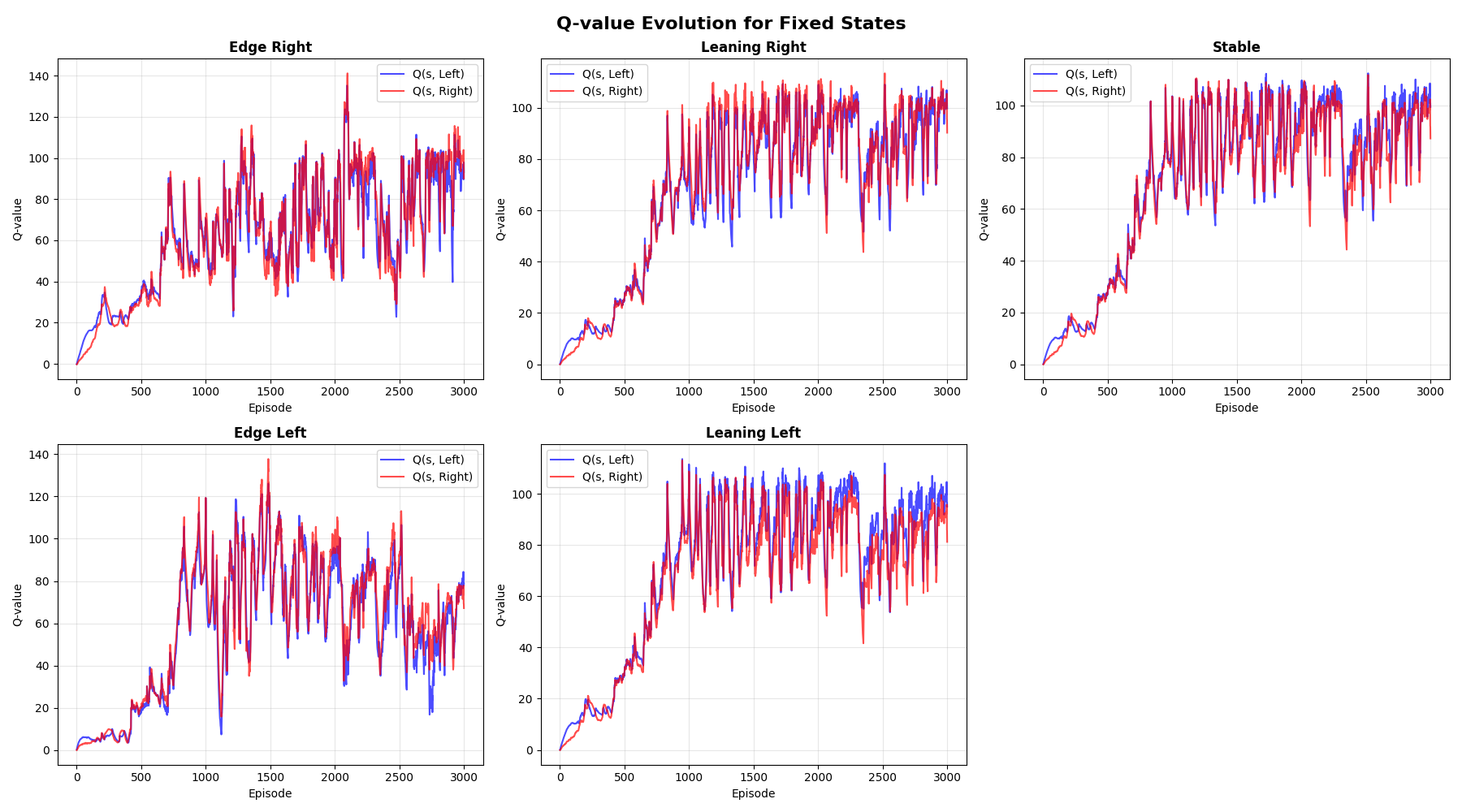
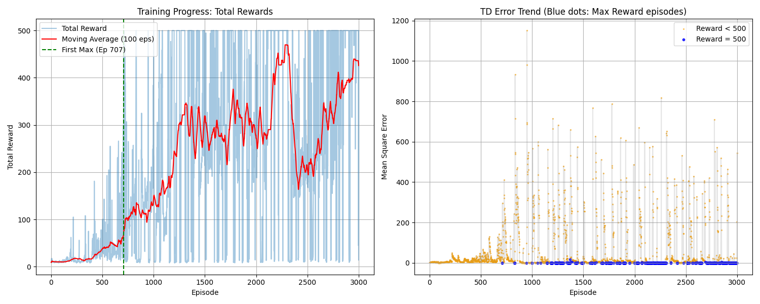
The results seem not that different from those of SARSA.
4. Q-learning with Experience Replay
Okay, I set the capacity of the replay buffer to 10,000, the batch size to 32, and the update (training) frequency to every four steps. Let’s see the results.
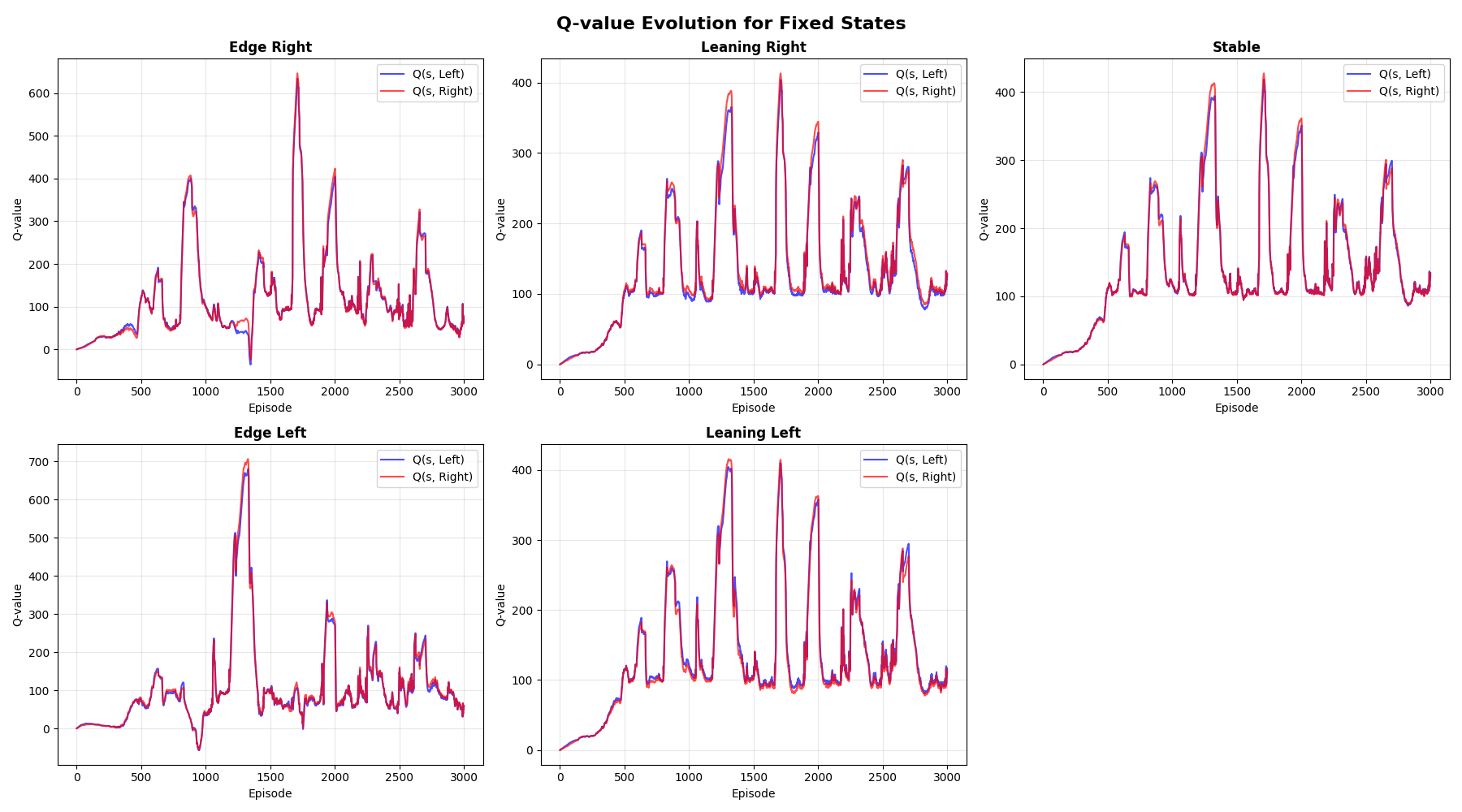
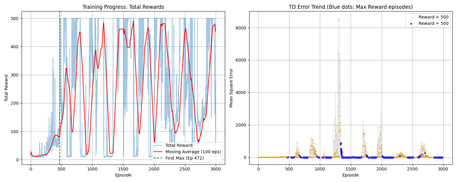
Surprisingly, many things changed. First, the episode-total reward plot became more stable (compared to before), even though periodic drops still occurred. This makes sense because gathering experiences from various episodes and using a batch of 32 leads to longer periods of stability (staying at the peak). However, this prolonged stability causes the replay buffer to be filled with only stable data, which narrows the buffer’s distribution. This is likely why we still see periodic drops.
Second, Q-values also stabilized relatively well, but there was a sudden spike. Let’s focus on episodes between 1200 and 1400. Total rewards dropped during that period, while the Q-values of the five fixed states skyrocketed. Why? Most likely, staying at the peak caused the buffer’s distribution to become too narrow, which in turn narrowed the Q-network’s coverage. At that point, when the Q-network encountered an unfamiliar state, such as leaning right, edging left, or leaning left, it incorrectly output a very high Q-value. Consequently, the Q-network learned that leaning right or left is a desirable state. Ultimately, this caused the total reward drop. (That’s my theory.)
So, the problem is still forgetting, which, I believe, cannot be solved by target networks, Double DQN, or Dueling DQN alone. Intuitively, even when the episodes become full of successful experiences, the buffer still has to keep unsuccessful experiences and how to recover from them.
5. Dual Buffer
The dual buffer idea is to separate successful experiences from unsuccessful experiences, and sample from them by a fixed ratio like 7:3. I think this could be a direct remedy for periodic drops. I set the capacities of the successful buffer and unsuccessful buffer to 5000 each, with the same batch size of 32. Let’s see the results.
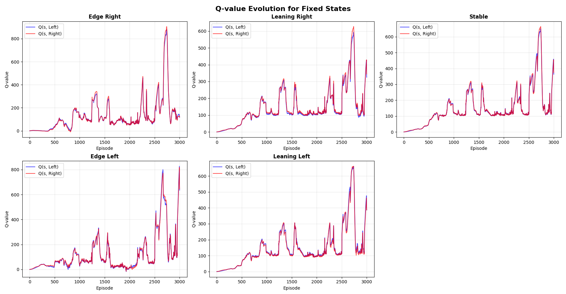
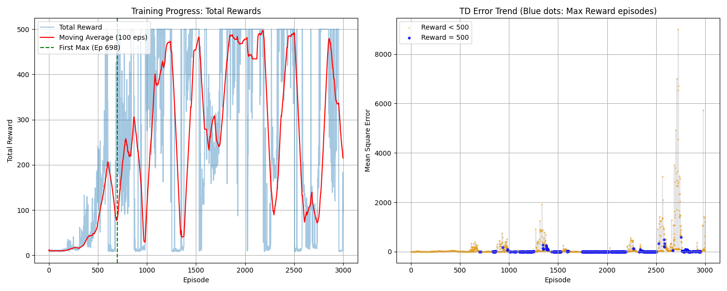
Logically, I believe adding a dual buffer was the right approach, but it hasn’t solved the periodic drop problem so far. In the meantime, the Q-values became too high and the TD error skyrocketed. I think we should solve this problem first.
6. Double DQN
The idea of separating the main Q-network and the target Q-network is a well-known solution for Q-value overestimation [3, 4]. The reason I didn’t use this idea earlier was that I thought the dual buffer could solve the periodic drop problem even without separating the Q-networks. Anyway, let’s see the results.
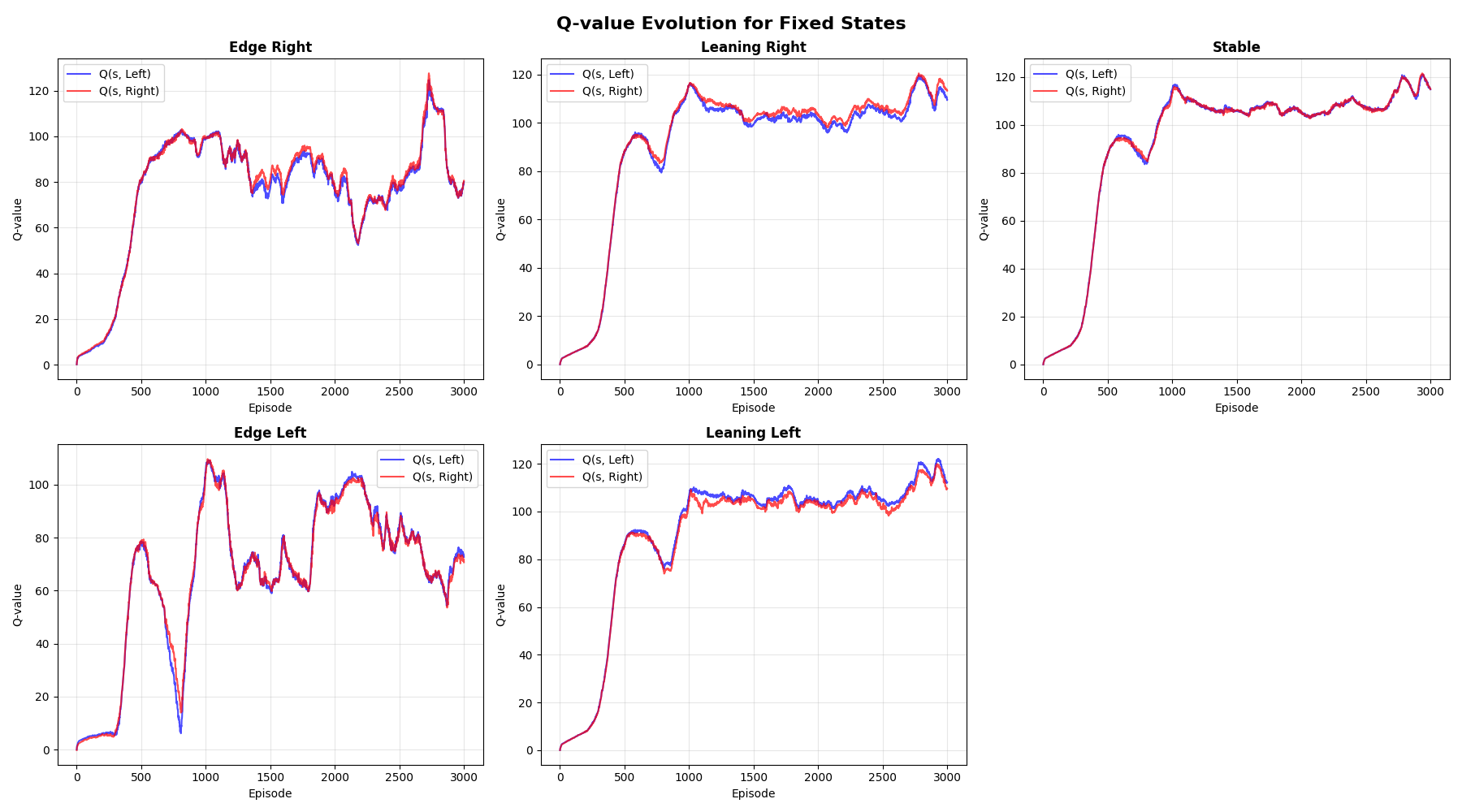
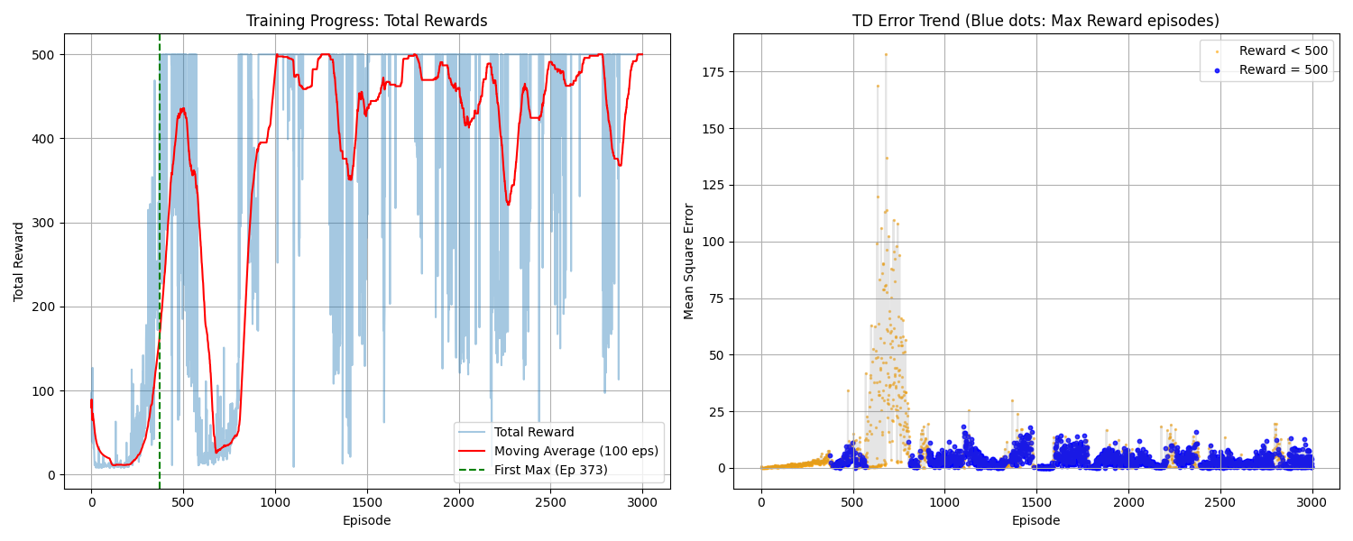
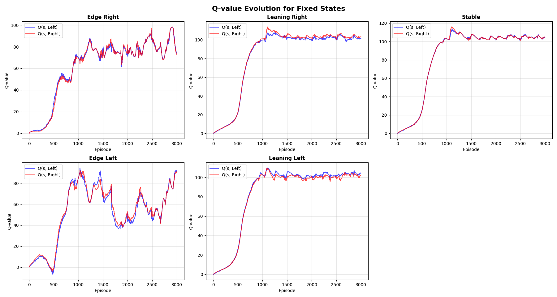
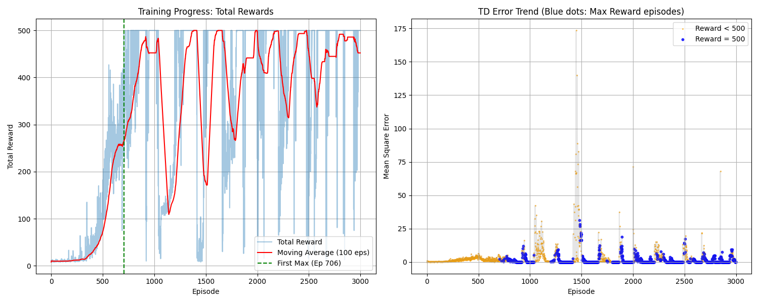
The results improved incredibly. Q-values stabilized, which caused the TD error to stabilize as well. Periodic drops are still there, but they have been somewhat mitigated.
So, why did it improve? By separating the main Q-network and the target Q-network, and updating the target Q-network slowly toward the main Q-network, we can mitigate the sudden overestimation of the main Q-network.
For example, even when the buffer is filled with 500-reward experiences, if the main Q-network encounters a forgotten situation, like leaning right, it might overestimate the Q-value. However, because the target Q-network is updated slowly, this overestimation can be mitigated. Specifically, with a soft update factor $\tau=0.01$, the target network only incorporates 1% of the main network’s weights at each step, ensuring the target values remain stable.
Click to see Double DQN without Dual buffer case
7. Refining Buffer Strategy
Back to the buffer
Okay, let’s go back to buffer modification. I noticed that the Q-values tended to drift upward as the steps progressed, which was especially obvious before implementing Double DQN. My theory here is that because I defined the “unsuccessful buffer” as simply the storage storing every state of episodes where the total reward was less than 500, the buffer eventually became saturated with “long” unsuccessful experiences.
Why could this be a problem? “Long” unsuccessful experiences (e.g., an episode lasting 400 steps) look almost identical to successful ones for the first 399 steps. Since the majority of transitions in these episodes still yield a reward of 1, the unsuccessful buffer begins to mirror the successful buffer, diluting the “failure signal” the agent needs to learn from.
If we look closely at the CartPole reward system, the environment outputs a reward of 1 for every step the cart remains upright and a reward of 0 only when it falls or moves out of bounds. This means 1 is the dominant reward, while 0 is extremely rare. So, the moment the environment outputs 0 is the only time a truly meaningful signal is transmitted to the network. It marks the exact transition that should be avoided. Therefore, when “long” unsuccessful experiences dominate the buffer, these crucial reward-0 transitions become even scarcer.
Failure Buffer
To fix this, I renamed the unsuccessful buffer to the Failure Buffer. Instead of saving entire “bad” episodes, I modified it to store only the specific terminal states where the reward is 0. By specifically sampling these “failure points,” we ensure the model constantly remembers exactly what “losing” looks like, preventing the distribution from narrowing too much even when the agent becomes highly skilled.
This approach is conceptually related to prioritized experience replay [5], which prioritizes transitions with high TD error. Here, we prioritize failure states (reward = 0) since they carry the most critical learning signal in CartPole’s sparse reward structure. Let’s check the results.
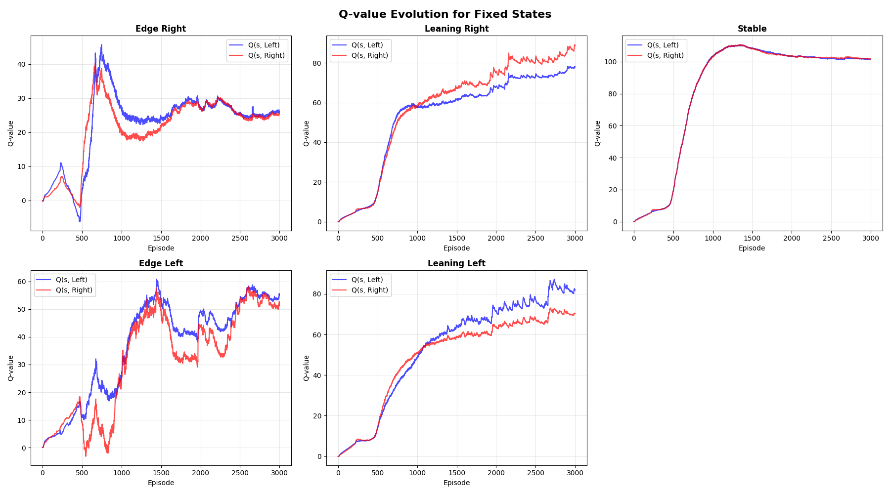
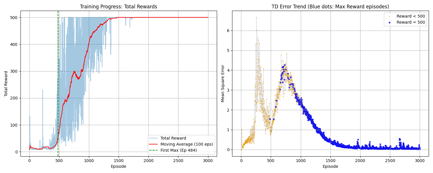
The total rewards plot looks perfect. The TD error is also decreasing smoothly like a loss plot in supervised learning. Q-values of action right and left are also visibly separated. And at the stable state, it merges to 100, which is intuitively and ideally correct, because I set gamma (discount factor) to 0.99. $1/(1-0.99) = 100$
However, it turned out that it was a lucky case. I did two more runs, and below are the results.
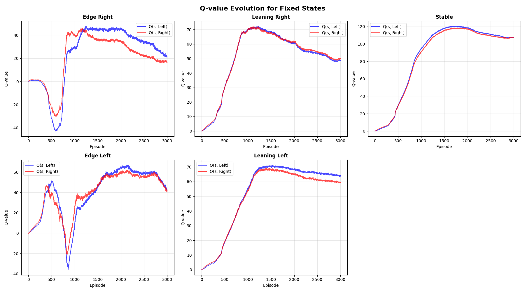
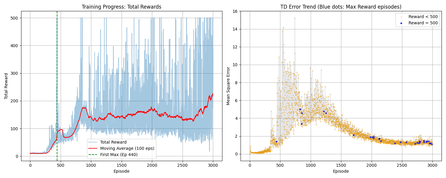
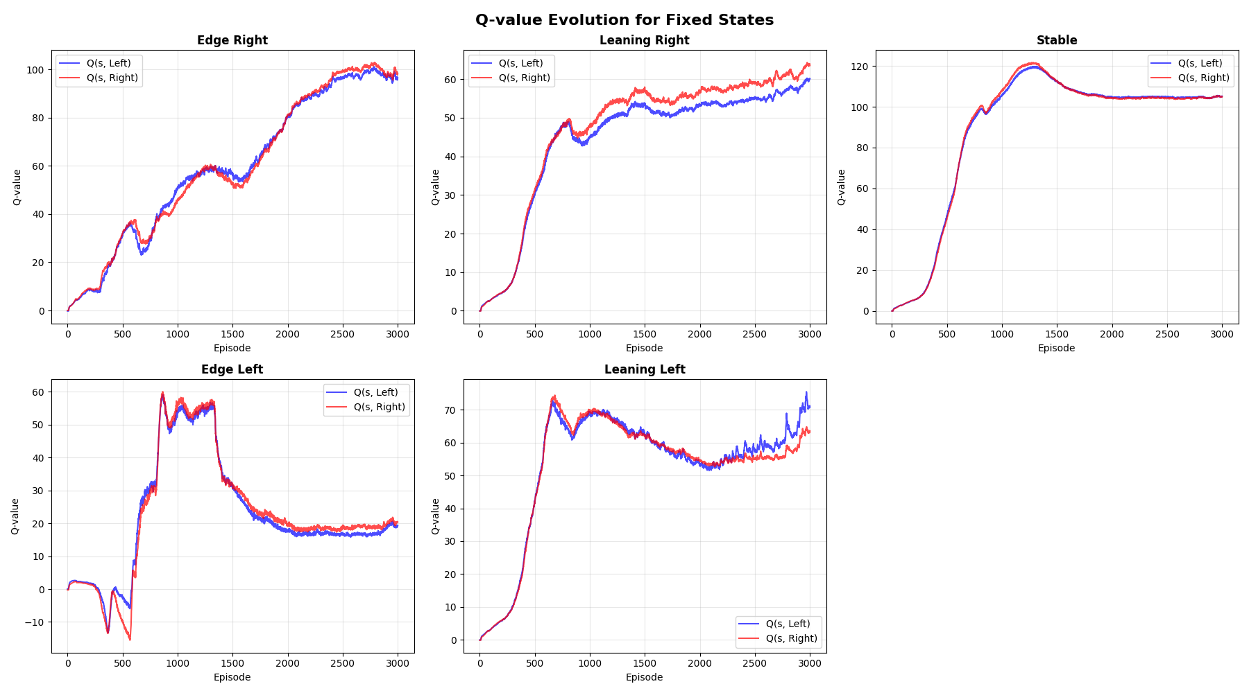
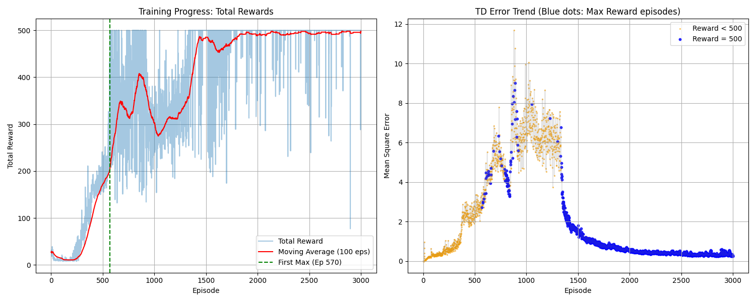
As shown in the upper figures, reaching a stable score of 500 could take a considerable amount of time. Also, the lower figures indicate that the performance remains somewhat unstable. Why? The first issue likely occurs because the Q-network learns primarily from two extremes: the successful and failure buffers. Consequently, the network struggles to bridge the gap between failure and success.
To avoid slow learning and to be more robust, I believe the Q-network should learn incrementally rather than attempting to jump directly from failures to ’lucky’ successful cases. To address this, I am considering removing the successful buffer and instead maintaining a “normal” buffer, which stores all states except for failures, alongside the failure buffer. This normal buffer could effectively facilitate the incremental connection between failure and success.
Normal Buffer and Failure Buffer
Let’s check the results.
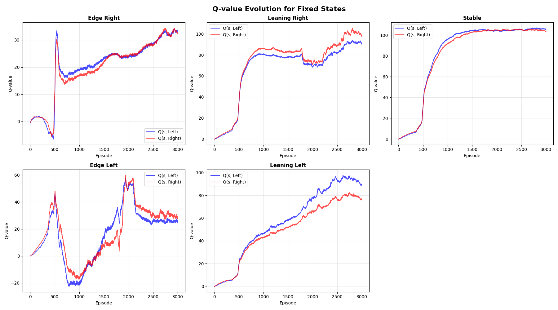
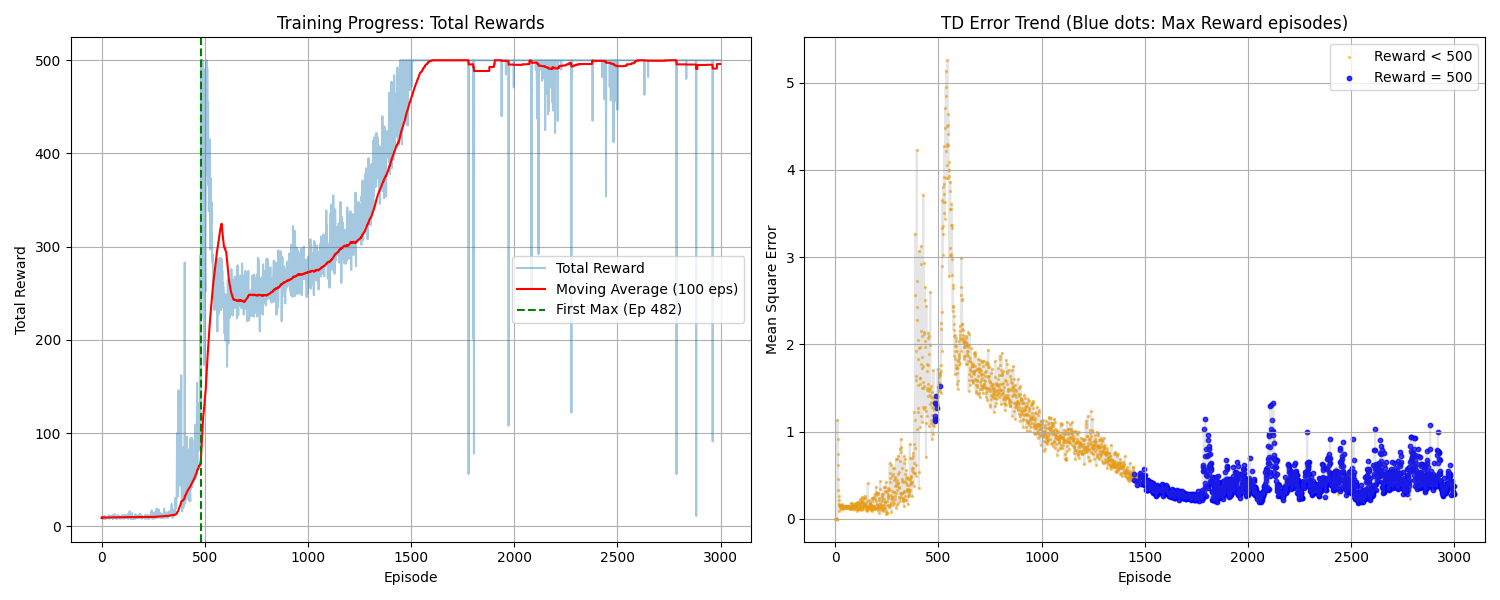
The plot looks prettier than before. I think this change is beneficial for two reasons. First, it prevents too-slow learning by incrementally connecting failed to successful experiences as I said. Second, it could also help recovery from significant weight changes, which I haven’t encountered yet.
Now, I think changing the sampling ratio from the two buffers, which was 7:3, might improve the stability.
Adjusting Sampling Ratio
Let’s try 6:4.
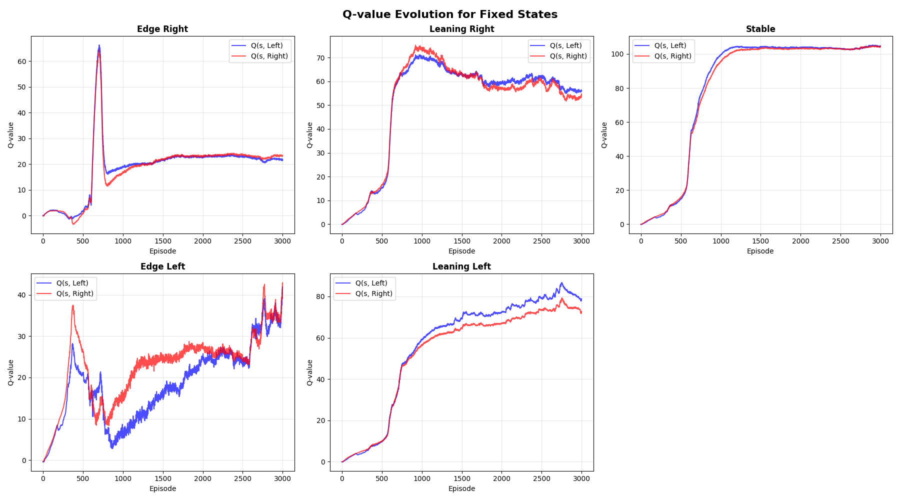
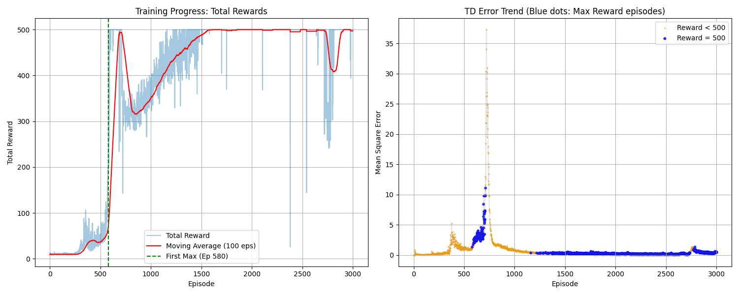
The results could be ambivalent. Let’s go back to 7:3. However, these results present critical insights. If we look at the episodes between approximately 2700 to 2800, there are suddenly many drops. Why? Below is the log of that range.
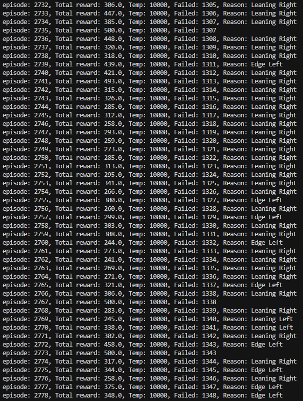
| Category | Count | Percentage |
|---|---|---|
| Edge Left | 33 | 2.4% |
| Edge Right | 679 | 49.9% |
| Leaning Left | 566 | 41.6% |
| Leaning Right | 83 | 6.1% |
This drop coincided with the agent encountering Edge Left and Leaning Right scenarios—classes that are significantly underrepresented in our current failure buffer (2.4% and 6.1%, respectively). This suggests that the model’s previous success was partly due to favorable sampling. Once exploration triggered these sparse failure modes, the agent lacked sufficient data in the buffer to recover quickly. Consequently, balancing the class distribution within the failure buffer is critical for robust learning.
However, I am concerned that further manual adjustment of the buffer might lead to excessive ‘hand-crafting.’ Well, I believe this is a good time to wrap up, and here are the takeaways.
Summary
- Achieving the maximum reward of 500 is relatively easy, and even SARSA or a naive DQN can reach this level.
- Experience Replay is highly effective for stabilizing training; however, without Double DQN (i.e., separating the online and target networks), it causes Q-values to grow uncontrollably.
- Double DQN appears to be essential when using Experience Replay, since standard Q-learning tends to overestimate Q-values beyond their theoretically correct range.
- Maintaining an additional failure buffer that stores only terminal transitions (state–action pairs yielding reward 0) proved effective for long-term stability, since CartPole’s reward signal is extremely sparse and failures provide the most informative learning signal.
- In one run, the episode–reward curve became nearly perfectly stable. However, this was likely due to overfitting to only one or two dominant failure modes, while the buffer at that time contained mostly “successful” trajectories.
- To become truly robust, the agent must learn to handle all four major failure modes (edge right, edge left, leaning right, leaning left). One promising direction would be to balance the failure buffer so that each failure type is represented evenly (e.g., 25% each), although this was not explored here. Additionally, 3,000 episodes may still be insufficient to fully achieve such robustness.
References
[1] Sutton, R. S., & Barto, A. G. (2018). Reinforcement Learning: An Introduction (2nd ed.). MIT Press.
http://incompleteideas.net/book/the-book-2nd.html
The foundational textbook covering TD learning, SARSA, and Q-learning algorithms.
[2] Mnih, V., et al. (2013). Playing Atari with Deep Reinforcement Learning. arXiv preprint arXiv:1312.5602.
https://arxiv.org/abs/1312.5602
Introduced Deep Q-Networks (DQN) with experience replay, demonstrating how neural networks can be stabilized for Q-learning.
[3] Mnih, V., et al. (2015). Human-level control through deep reinforcement learning. Nature, 518(7540), 529-533.
https://www.nature.com/articles/nature14236
Extended DQN work published in Nature, providing comprehensive analysis of experience replay and target networks.
[4] Van Hasselt, H., Guez, A., & Silver, D. (2016). Deep Reinforcement Learning with Double Q-learning. Proceedings of the AAAI Conference on Artificial Intelligence, 30(1).
https://arxiv.org/abs/1509.06461
Introduced Double DQN to address Q-value overestimation by decoupling action selection and evaluation.
[5] Schaul, T., et al. (2016). Prioritized Experience Replay. International Conference on Learning Representations (ICLR).
https://arxiv.org/abs/1511.05952
Proposed prioritizing transitions based on TD error, related to the failure-focused sampling approach used in this post.
[6] Gymnasium Documentation (formerly OpenAI Gym). CartPole-v1 Environment.
https://gymnasium.farama.org/environments/classic_control/cart_pole/
Official documentation for the CartPole environment used in these experiments.